Abstract:
In my second bachelor thesis, I explored the usefulness of applying static filters, i.e. the Scattering Transform to object detection. I found that the Scattering Transform has desirable properties w.r.t. some equivariances and in the low-data regime. In all other cases, no beneficial properties of the Scattering Transform have been found.
1. Introduction
There are many unknowns in the training of any deep learning architecture. We have no guarantee that it converges to a reasonable optimum, we don’t know after how many steps it converges and we can’t really predict what features the filters in Convolutional Neural Networks (CNNs) will learn. In practice, we circumvent these challenges by training with multiple different hyperparameters and using other heuristics to improve training. Optimally we want to make sure that a network fulfills some theoretical guarantees after training, i.e. equivariances. Equivariance, in the context of this post, just means that if a transformation is applied on an object in an image we want the network to be able to still detect that object correctly. This is especially important in the context of self-driving cars. If the position, size or orientation of a pedestrian is changed we want to have the guarantee that they are still detected correctly. In this thesis, I tested whether using static filters that are known to have some of these desirable properties in combination with current Deep Learning frameworks yield the desired effects.
2. What is the Scattering Transform?
The paper that introduced the Scattering Transform makes it sound way more complicated than it really is. The scattering transform is just the application of multiple filters on an image in a particular fashion. The filter is a Morlet wavelet (also known as the Gabor filter for people who come from a Neuroscience background). This Morlet wavelet/Gabor filter is a product of a sinusoidal wave with a Gaussian. A mathematical definition is intentionally left out because I think it is more confusing than helpful (see Morlet Wavelet Wikipedia). It looks like this in 1D:
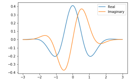
Even though the theory might look complicated I think it is easiest to think of the Morlet wavelet as some kind of ‘fancy’ edge detector. It comes with some additional properties but from the 1D image alone it is clear that the filter mostly finds gradients along some axis. The main idea of the Scattering transform is to apply this filter multiple times, i.e. in different angles and sequentially. The sequential application of two filters can be seen as a layer in a network. For example, we can have a two-layer Scattering network with four angles. That means we have 4 filters in the first layer and 4*4 in the second. Even though the network is built in a ‘pipeline’ fashion the output of every filter at every layer is relevant and used. This is the case because further applications of the Scattering transform yield more specific features unlike in a conventional CNN where additional layers become more general and abstract. In our example, we would, therefore, have 1 + 4 + 16 outputs. These 21 outputs can be interpreted similarly to 21 features in the early stages of a CNN. The one filter in the zeroth layer is a low-pass filter that is applied before the remaining transformations. A sketch of a network is shown in the following figure:
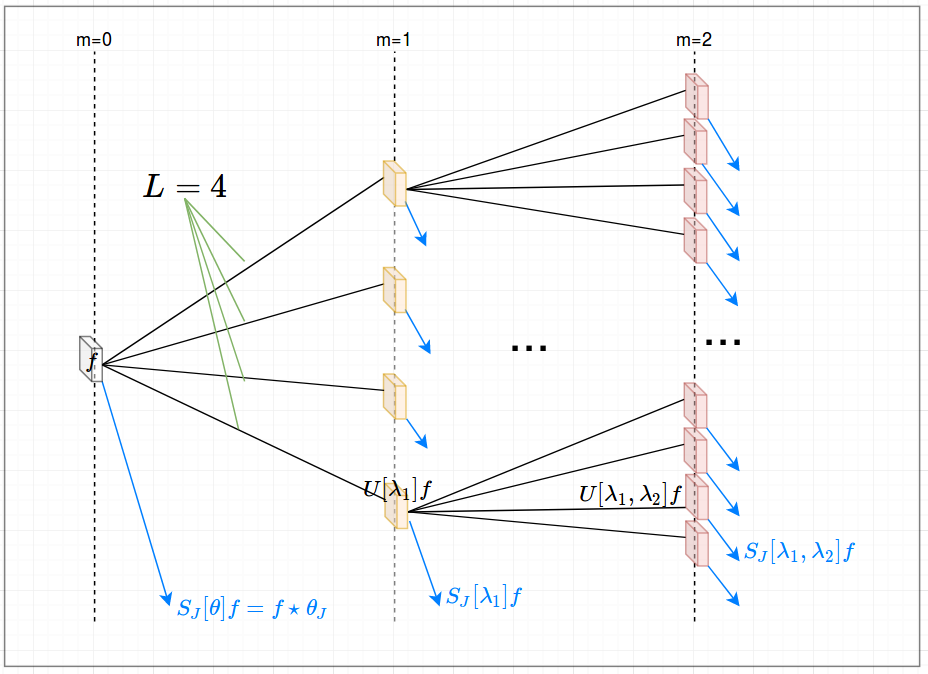
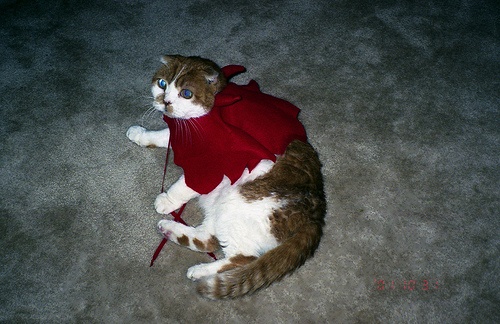
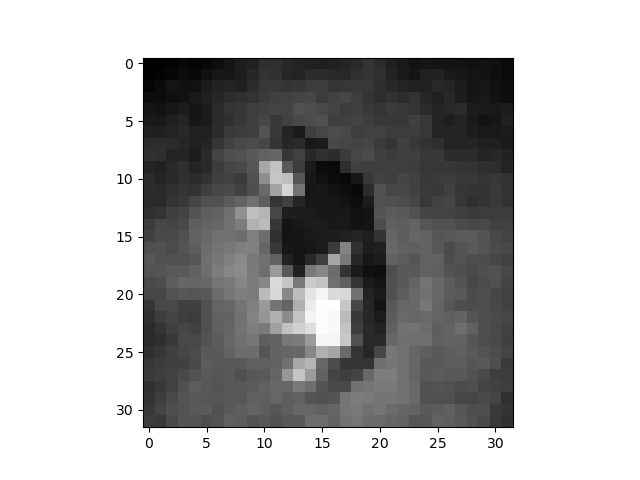
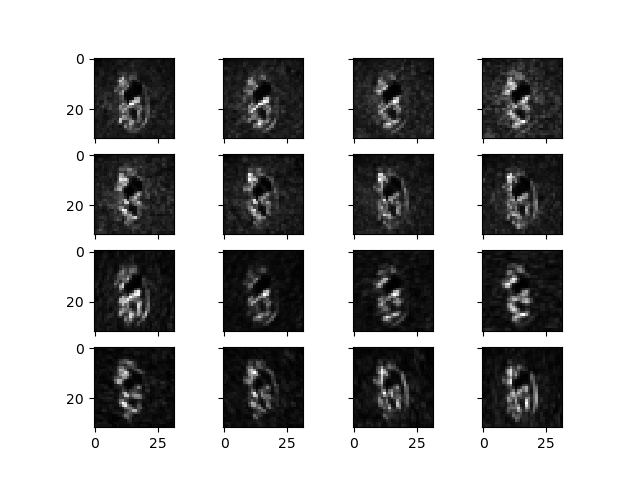
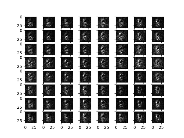
To give a better understanding of how the Scattering transform looks at different stages of the network I show the outputs of different layers of a 2-layer Scattering Network applied on the image of a cat. Layer 0 is just the application of a low-pass filter that removes all high-frequency waves from the image. It just makes the image a bit more blurry. Layer 1 shows 16 different outputs after the first application of a filter. The reason why there are 16 outputs is because in this setting we have 8 different angles and 2 different sizes of outputs. Layer 2 shows 64 different outputs after the second application of all filters. If we look carefully at the outputs of layer 1 and 2 we see that the difference is only marginal and not worth the computational cost or the space in memory. Therefore we used one layer Scattering Networks in most of our experiments.
A scattering network alone is probably pretty useless for detection purposes because it requires handcrafted features that are known to be worse than very simple CNNs. We, therefore, want to combine the theoretical guarantees of the scattering transform with the flexibility of Neural Networks to get the best of both worlds. These combinations are called hybrid networks in the context of this paper.
3. Experiments
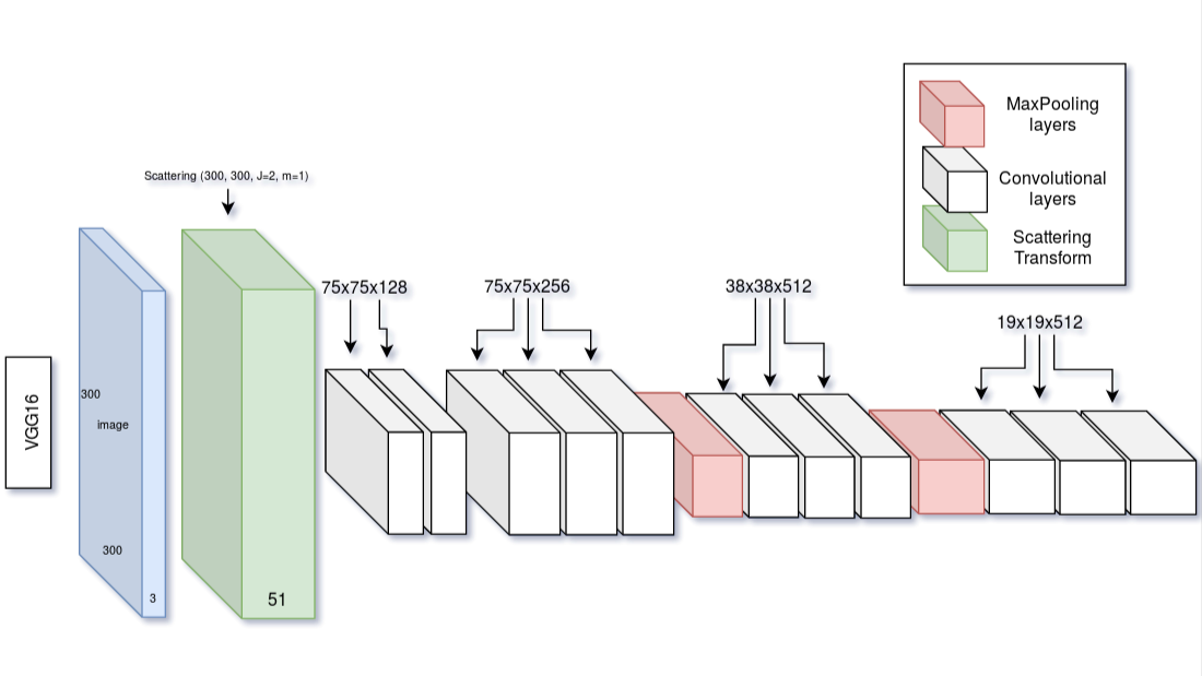
In our first experiment, we tested the combination of scattering and conventional neural networks in two ways. First, we combine the networks sequentially, i.e. every image has to first pass the scattering network, the output of which is the input for the rest of the network. Since the scattering network fulfills the same functionality as the early layers of a CNN we just remove some of them. For the object detection network, we chose the Single Shot Multibox Detector (SSD) since it is a fairly simple but fast detector. A visualization of the sequential scattering architecture can be found here:
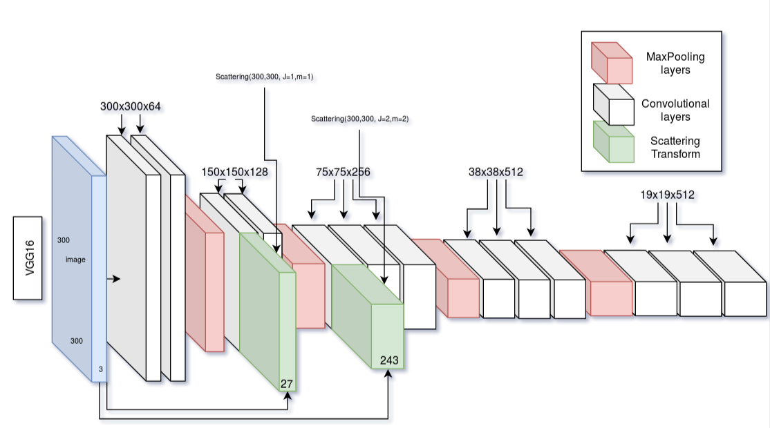
The second idea was to combine the networks in parallel, i.e. just merge the filters of the two networks at different stages of the pipeline as shown in the ‘Parallel Scattering SSD’ figure. This was intended to make sure that robust features exist at every step of the training but also have the flexibility of the learning filters.
Lastly, we performed some experiments on training time, behavior in the low-data regime and on specifically designed toy datasets that each inspect the behavior of the network w.r.t. one particular transformation (scaling, rotation, translation, deformation). For natural images, we used the Pascal VOC and Kitti dataset. Pascal VOC contains everyday scenes containing one object. On rare occasions, more than one object is included in an image. Because of these properties, Pascal VOC is a fairly easy object detection task and we would expect good performance on it. Kitti contains images of traffic scenes that can contain many objects such as cars, cyclists or pedestrians. Most of the time an image on Kitti is far more complex and contains more objects and therefore we expect the network to perform significantly worse on it.
4. Results
Most of the results can be summarized by looking at the following figure:
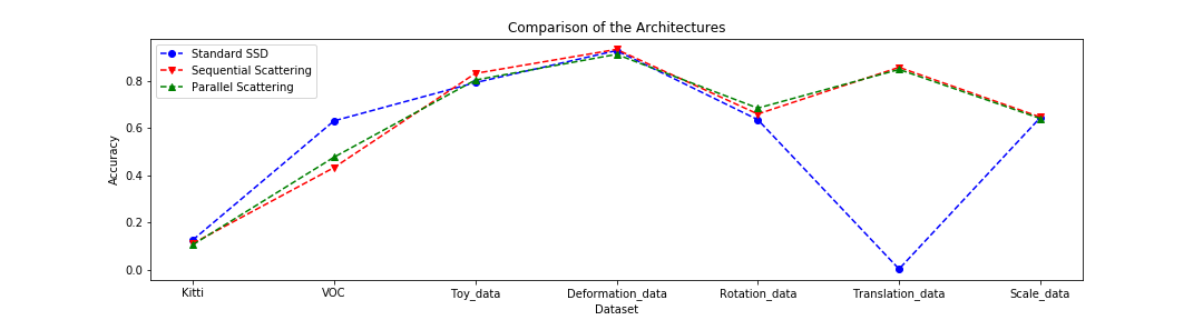
We can already see that all architectures perform pretty similar on all but 2 datasets. On VOC the vanilla SSD outperforms the hybrid networks and on the translation toy dataset the vanilla SSD completely breaks. Further experiments that I conducted after the deadline had already past and the thesis was handed in showed that I had made an engineering mistake and also in the case of the translation data the performance is, in fact, similar to hybrid networks. The experiments that were conducted in the low-data regime also turned out not to show any tangible benefit of the scattering architectures. We could show that the forward pass of the sequential scattering hybrid is 25 percent faster than the one of a vanilla SSD but that is only a minor benefit.
5. Conclusions
Scattering hybrid networks use static filters for the first couple of layers of CNNs. While they are faster because they need less training and have some nice theoretical guarantees such as behavior w.r.t. equivariances the results turn out to be disappointing. The parallel architecture is significantly slower w.r.t. training time than a vanilla SSD and has no benefit whatsoever. The sequential architecture is slightly faster per forward pass but also shows no tangible benefit other than that. Especially when natural images are concerned, such as in the Kitti dataset, the vanilla SSD outperforms both scattering hybrids. This is likely the case because the features in natural scenes require more than ‘fancy edge detection’. Additionally, SSD is a very simple detection network. More advanced networks such as Faster-RCNN or Masked-RCNN probably use more complicated internal representations and their performance will drop even more drastically by combining them with static filters. Overall I think this is a method that should only be used in very niche situations. The only situations that I could imagine this being useful are low noise environments where the high tempo is an advantage. An example could be sorting good and bad apples on a production line.
One last note
If you have any feedback regarding anything (i.e. layout, code or opinions) please tell me in a constructive manner via your prefered means of communication.