Abstract:
In my first bachelor thesis, I tested whether “inverting” the classification process by using gradient information of generative models is effective. One of the problems turned out to be that the latent space became less structured for larger datasets and the results, therefore, got worse. In a follow-up study, which yields the content of this post, we found that using expert modules removes this problem and yields better results on sparse datasets. The paper has been accepted for publication at the European Symposium for Artificial Neural Networks (ESANN) and you can find the paper in its proceedings.
1. Introduction
As already discussed in my previous blog posts on Inverse Classification (part I, part II) that the Cognitive Modelling group in Tübingen around Martin Butz and Sebastian Otte is very convinced of the hypothesis of The predictive mind (I find it very plausible as well). In short, it states that the mind is to a large extend predictive, i.e. instead of reacting to your surroundings and building your mental model around it your brain predicts it’s surroundings and only updates this model slightly through the perceptions you have. The first and second post have focused solely on the predictive part of the brain but this part includes an additional aspect, namely modularity. The brain is not just a random collection of 86 Billion neurons with connections between them but it is highly specialized and modularized. A lot of functionality can be attributed to specific regions of the brain (e.g. vision to the visual cortex) and, thereby, is an interplay between different ‘experts’.
In part I we found that the predictive hypothesis seems to hold very well for a small number of classes but as soon as you scale up the experiments the tasks seem to get too complex. To contain the complexity we introduced modules/experts for every single class that we want to predict.
2. Setup
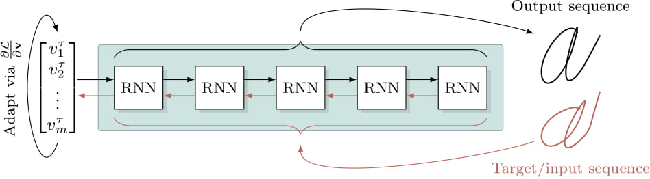
In the standard classification setup you get an input, you forward it through your classification pipeline and you receive a probability vector over class labels. In the Inverse Classification setup used in this post, instead of forwarding the image through the network, you try to generate a similar image from a probability vector. You start with a uniform vector, generate an image, compare this image to the target and backward the loss via any gradient descend method (we chose Adam). The newly updated class probability vector is forwarded again and a new prediction is generated, compared to the target, the loss is backwarded, until, hopefully, you converge to a final probability vector. The general concept is visualized in the following figure.
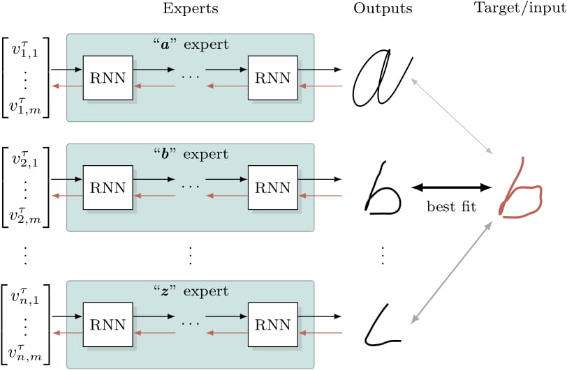
The specialty in this setup is that every class has its own expert module instead of one big network for all classes. The experts compete against each other in the sense that they are able or unable to create a sequence that resembles the target and therefore have a higher or lower loss. The competition is won by the network which yields the lowest loss. To clarify consider the following figure.
3. Experiments and Results
While this methodology could in theory be used with any dataset and generative network we have chosen an LSTM since we work with sequential data. The datasets we use are handwritten digit sequences from the UCI repository and MNIST in the sequential interpretation, i.e. instead of interpreting it as a 2D matrix we view MNIST as a sequence of 28-dimensional vectors that are fed into the network sequentially. As I have already discussed in the second part, this technique is already very good in the low data regime but does not improve that much with more data. To find out how good exactly it is with few data we have focused our efforts on the low-data regime. More specifically, this means four data points per class resulting in 40 training points for MNIST and 80 for the handwritten digits.
How good is the Generative Network?
Before we analyse the actual classification results we should investigate how well the invididual expert modules generate their respective letters. If the generation is bad already, Inverse Classification is likely to fail anyway. For this reason, we have cherry-picked some generated results to highlight noteworthy things. In the following two figures you can see the four training points in the top row, the targets in the second, and the results of the Inverse Classification for that expert in the third. It is important to note that the four sequences in the top are the only data points the network has ever seen during training.
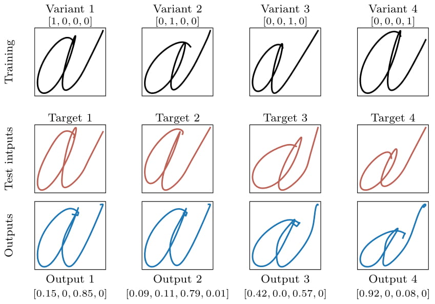
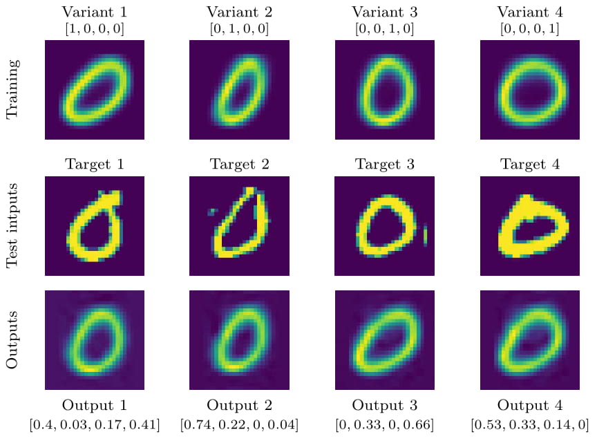
From these figures we find two important observations: a) The networks are able to recreate/generate sequences they have not seen during training. This becomes especially visible in the third column of the characters figure. Target 3 has a bend in the right-hand tail of the ‘a’. This bend can’t be found in any of the training points and yet the network is able to create it from gradient information alone. b) The expert modules use combinations of existing knowledge and characters to create these new and previously unknown targets. These combinations might not be interpretable by or feel natural to a human but at least they recreate the desired goal sufficiently well. These two observations are the crucial necessary components for the rest of the experiments as the classification would otherwise just be template matching.
How good is Modular Inverse Classification?
To evaluate our method we have to look at experimental results. Before we do that, though, we test how well ‘calibrated’ our expert modules are, i.e. how well they are able to classify their own and only their own class. If we have a very powerful generative network that can also recreate other classes the entire idea of experts would collapse. On the other hand, we want to make sure that our experts are flexible enough to account for in-class variance, i.e. they are able to recreate different types of the same class. To test this notion of calibration we created heatmaps for both datasets. The heatmaps show the average loss (mean squared error) for all combinations of experts and data points. The cell (0,3) in the top row, for example, shows the loss of the 3-expert for class 0. We apply this procedure for the training data (left) and the test data (right) on MNIST.
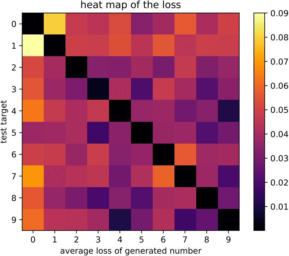
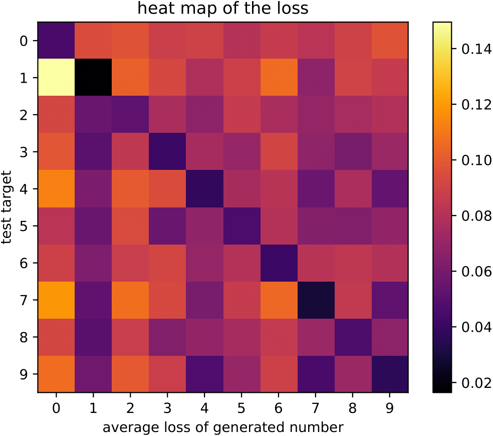
We find that the experts are mostly well-calibrated. In the case of the training data, the black diagonal indicates that our experts recreate the training data very well while not being able to generate other classes. The same effect can be seen for the test data, even though in slightly weakened fashion - even with the test data (e.g. data that the networks haven’t seen before) the training loss for the correct class is always the lowest.
The figures have given us a rough intuition about the performance of our method so far but we would also like to have some quantifiable comparisons. The experiments conducted in the paper are all in the low-data regime as we have found in previous experiments that the Inverse Classification approach is particularly suited for it. We compare the modular approach, or Ensemble of Generative Expert Modules (EGEM), on two datasets using different methods and setups. The two datasets are MNIST and a set of handwritten letters. Importantly, since we use RNNs, the datasets are represented as sequences not as 2D images. As we are in the low-data regime we only use 4 data points per class. We test two different methods to choose the 4 data points per class: a) randomly (‘random’) or b) we cluster the data with k-means clustering and choose the cluster representatives (‘clustered’). The two conditions are supposed to represent different real-world scenarios. Per dataset and condition we compare five different scenarios: a) EGEM without any addition (‘base’), b) EGEM that was trained with the addition of noise (‘noise’), c) the best model of the noise scenario (‘best’), d) Using a similar LSTM to classify the data in a forward fashion (‘forward’), and e) a nearest neighbor (NN) approach which is known to yield solid results on small and simple datasets. We also include a comparison with an LSTM forward classifier that is trained on the entire dataset.
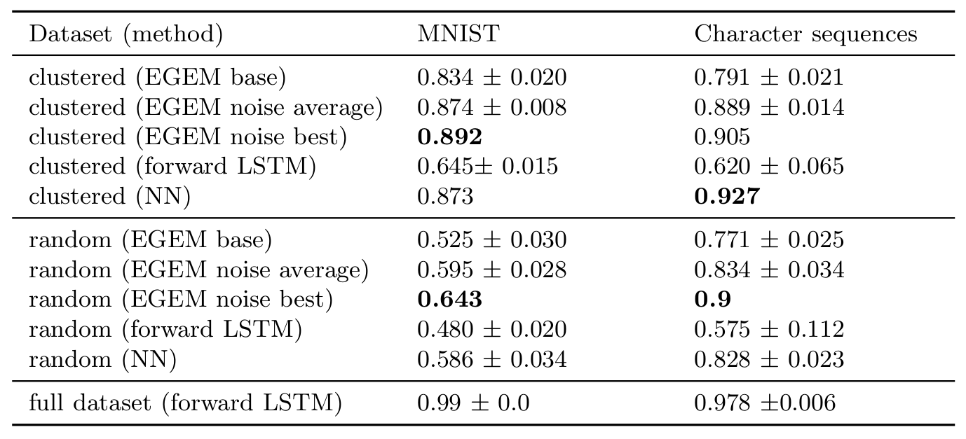
We find firstly, that the inverse modular approach is always better than the forward LSTM approach by a significant margin (10-20 percentage points). This is already some evidence in favour of the modular approach. We find additionally that in 3 of the 4 scenarios both the average and the best network from the noise condition beat the nearest neighbor classifier. It has to be pointed out though, that the datasets we use are rather simple and more complicated scenarios might look entirely different.
4. Conclusions
From my personal perspective, the advantages of the combination of Inverse Classification with Expert Modules are a) it seems to work fine in the low-data regime and b) It has high interpretability as you can easily test which expert yields which best guess.
On the other hand, it also comes with some problems. Firstly, it does not scale to larger datasets unlike most other ML methods (at least in our setup) which makes it a rather niche application. Secondly, it is restricted to datatypes that actually have a good distance function since there is no possibility to update and iterate otherwise. While mean-squared-error might still work for MNIST it can’t handle CIFAR or more complicated image data. Lastly, it is a rather slow process. Every classification includes multiple backward and forward passes and thereby increases the speed of classification dramatically. At this point you can honestly just use a Gaussian Process and use its advantages like actually giving meaningful uncertainty estimates.
As you might have noticed I’m not particularly sold on the current applicability of the method. However, I think it has lots of potential and the general direction of using generative models for more applications is really interesting. My supervisor for this project, Sebastian Otte does a lot of research in this direction with significantly more impressive results. If you find this interesting I can wholeheartedly recommend reaching out to him. He is a great supervisor.
This is the last post on the topic of Inverse Classification since I have moved to a different group at the University of Tübingen for my Ph.D. Posts of my current work are already in the making.
One last note
If you want to get informed about new posts you can subscribe to my mailing list or follow me on Twitter.
If you have any feedback regarding anything (i.e. layout, code, or opinions) please tell me in a constructive manner via your preferred means of communication.