Abstract:
In my first bachelor thesis I tested whether “inverting” the classification process by using the gradient information of generative models is effective. After many experiments the conclusion is confirming the expected: it depends on the quality of the generative network. The better the generative network the better its ability to classify.
1. Introduction
My supervisor for the project, Sebastian Otte, and the Professor of the research chair, Martin Butz, have already conducted multiple experiments on gradient based methods in general. The motivation for using gradients for classification tasks comes from two hypotheses: 1. It is more robust against adverserial attacks. If you think of a trained feed-forward network, i.e. a CNN, as a very complex lookup table that also often overfits on meaningless features or proxies instead of the best possible features I think it becomes more plausible why they are so prone for adverserial attacks in the first place. A generative model has to develop some sort of inner representation of the concept it is generating and might therefore be less prone to these attacks. However, recent research suggests that this hypothesis is wrong. 2. Coming from a Cognitive Science background, I was also interested in understanding an modeling the brain. Most learning systems are not just a one way forward pipeline but rather a very interactive process in which information is propagated forward and backward multiple times. A particular framing that is often used (and I personally find very convincing because it explains so many biases or behaviour patterns of humans) is the following: The brain is mostly a generative model that constantly makes predictions about the real world and updates them given input data through the senses (also knowns as `the predictive mind’). Inverse classification probably is the most basic experiment one can conduct to test a very simplified version of this hypothesis. Given that this work is the first using temporal gradients for classification a lot of exploratory work is done, i.e. analysis of its capabilities and methods to increase its functonality.
2. What is Inverse Classification?
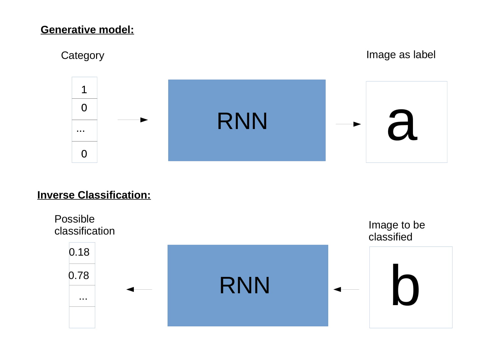
Inverse Classification is a two step process. In the first step a generative model is trained on a given dataset. This can be any generative model, i.e. it could be a generative adverserial network (GAN), a Variational Auto-Encoder (VAE) or any other. In this thesis we used LSTMs because the dataset we were using consisted of long sequences. The training is done until a good representation of a concept is learned. In our case the model was trained until the network has learned perfect representations of all classes. We used one-hot encoding for the classes, so inputting a vector that is one at its first entry and otherwise zero would, for example, generate the character ‘a’. In the second step the generative model is used to classify previously unseen data by iteratively updating its prediction using the temporal gradient information. This is done by starting with an arbitrary initial vector and generating a sequence from it. Given that we have no idea what our class is going to be, a uniform vector is the most plausible choice for initialization. The uniform vector generates a sequence which is then compared to the actual classification target. The error between prediction and target is calculated and backpropagated through the network yielding a gradient. This gradient can be used to update our initial guess, i.e. the uniform vector. This new vector can then be pushed forward through the network again and produces an output that is a little closer to the actual target. This iterative process can be done until the error between true target and reconstruction converges. At the point of convergence the input vector is taken as the classification and the class can be determined by using the maximum entry of this vector. If the vector has not converged to a one-hot it also gives valuable insight about what the network `thinks’ that the target is. So, for example, the character ‘a’ might be partly reconstructed using a ‘d’. An example of the entire process can be seen in the following figure:
3. Experiments
We conducted many different experiments with the aim to increase the accuracy of the Inverse Classification process. If you want to see them all you can check out the full thesis. The short summary is: all but one mechanism that we tested didn’t work but the successful one worked pretty well. A simple description of the working mechanism : we add Gaussian noise to the inputs before doing a training iteration and then clipping and normalizing the vector such that it still resembles a vector of probabilities. For example, a vector with four classes resembling an ‘a’ would look like this: [1,0,0,0] before the addition of noise and could look like this: [0.83, 0.06, 0.04, 0.07] after it. The whole idea of the experiment is to introduce some variability in the latent representations that the network sees during training and is therefore able to use during the Inverse Classification. Intuitively speaking: if the network has only seen one-hot vectors during training it does not know how to reconstruct a target using anything else. An additional variable that was controlled for within the experiments is the number of available training data points. Conventional forward networks are known for working well with huge amounts of training data and badly with few examples. In comparison, generative models are known to already perform reasonably well at lower amounts of data.
4. Results
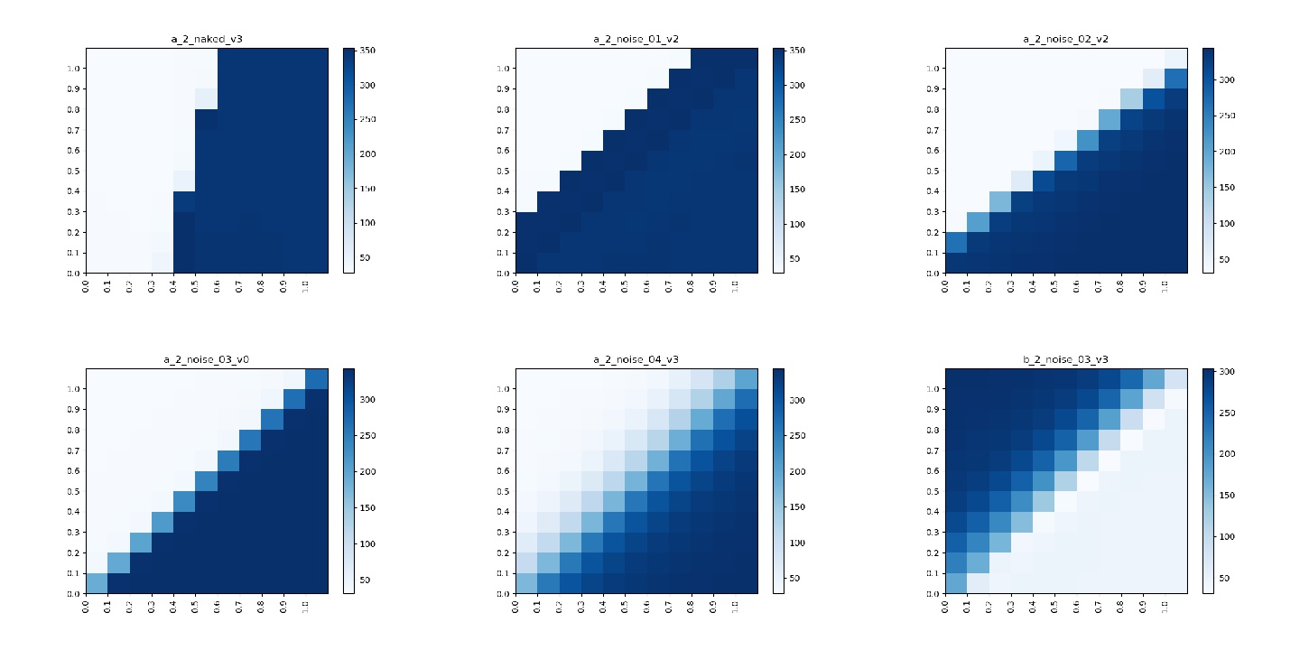
The first result is with regards to the addition of noise to the inputs. I have already hinted in the Experiments section that it was the only experiment with positive results but I want to show this in a more graphical fashion. In the following we consider a model that was trained on only two different character classes, i.e. ‘a’ and ‘b’. To test the influence of the addition of noise on the latent space of the model we did a grid search over a 2D grid with vectors ranging from [0,0] to [1,1] with steps of size 0.1 and plot the mean squared error to a stereotypical ‘a’. This means the heatmap is light when the model predicts an ‘a’ and gets darker the more different the predictions get from an ‘a’. If the latent space is perfectly separated our model would always predict the class which has the maximum entry in the vector, e.g. a [0.3, 0.8] would be predicted as ‘b’ and [1, 0.5] would be an ‘a’. The results for different models are presented as heatmaps in the following figure. A model with perfectly separated latent space has a decision boundary on the diagonal because this is where the maximum entry switches classes. In the first heatmap a vanilla model is presented, i.e. a model that is trained without the addition of noise to the input. In the following four heatmaps different levels of noise were added. Given that we add Gaussian noise, the levels just encode increasing standard deviations, in our case: 0.1, 0.2, 0.3 and 0.4. The last heatmap shows the mean squared error for the character ‘b’ of the 0.3 standard deviation model. This is shown to double check that the model not only has a good latent space for both classes but also no weird artifacts. This can be seen by overlaying (i.e. adding) subfigure 4 and 6. Combined they yield a smooth surface without any empty spaces, implying a smooth latent space.
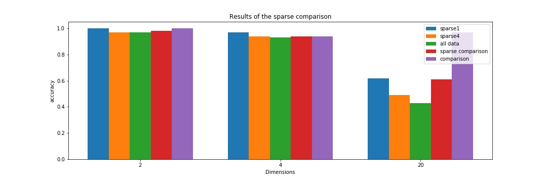
The second result concerns the amount of datapoints that was used for training. Five different scenarios with different amounts of data or settings were considered. In the ‘sparse1’ setting there was only one sample per class for training while there were 4 samples for the ‘sparse4’ setting and the full training set, i.e. around 220 samples per class for the ‘all data’ case. The accuracy of these models is compared to a conventional feed forward model trained on the entire set and one trained on 4 data points, namely ‘comparison’ and ‘sparse comparison’. The following figure compares all accuracies and tells a very simple but surprising story: In simple settings, i.e. a problem that has only 2 or 4 classes, it does not really matter what method you choose and how many training points you use. So even a model that was only trained on one example per class is just as good as one that was trained on multiple hundred training samples. The more complex problems, i.e. 20 dimensions get more interesting. The forward model trained on all data points outperforms every other approach by a big margin. The Inverse Classification models get better the less training data is used (This is especially surprising). I think the reason for this behaviour is an intrinsic problem with Inverse Classification, namely that every generative model holds exactly one representation of a class. I hypothesise that an inverse model trained on multiple representatives of a class might hold a weird ‘average’ of the samples that is a less good representation than just one sample. An inverse model trained on few data points is just as good as a forward model trained on few data points as can be seen with the ‘sparse1’ and the ‘sparse comparison’ accuracies. This, at least for me, is good evidence for the fact that Inverse Classification has potential as a technique, especially in the low data regime.
5. Conclusions
Honestly, I am not yet decided on the applicability of the Inverse Classification technique. I would argue that this basic research shows that it has some potential, especially in the low data regime. I think the two directions one would have to check to make a more informed decision are either a) to improve the generative model or to b) reduce the problem complexity in some way. For the first I could imagine using GANs to train the generative model instead of LSTMs. LSTMs are just not the state of the art of generative models and the GAN community has produced some astonishing results over the last few years. For the second option I could think of using a modular approach to Inverse Classification, i.e. using multiple smaller generative models and have them compete against each other to produce classifications. However, even if a better generative model might make the technique feasible there is one downside that might kill its practical application entirely. Since every classification process is an optimization in itself, there is a high computational overload attached to each classification step. This might not be much of a problem given that computing is faster and cheaper than ever but is only worth the extra effort if the results clearly outperform other methods. My most reasonable estimation of the technique is that it will probably be relevant for some niche applications but will not revolutionize the way we classify in general.
One last note
If you have any feedback regarding anything (i.e. layout, code or opinions) please tell me in a constructive manner via your prefered means of communication.