What is this post about?
I have been slightly confused about combinations of random variables (RV) in contrast to combinations of probability density functions (pdf). If we have, for example, two Gaussian random variables \(X_1\) and \(X_2\) then their sum \(W=X_1+X_2\) is again distributed according to a Gaussian. The sum of their pdfs \(p(x_1) + p(x_2)\), however, is not Gaussian. In contrast, the product of two Gaussian random variables \(Z = X_1 \cdot X_2\) is not Gaussian but the product of their pdfs \(p(x_1) \cdot p(x_2)\) is proportional to another Gaussian.
In this post, I want to clarify this confusion. I explain the differences between sums and products of RVs and pdfs using the example of Gaussians. Since I personally think very visually, most concepts are also shown through figures.
If you think I got something wrong or want to suggest feedback just contact me. Check out the accompanying GitHub repo if you want to play around with the code.
Notation
I’ll briefly define RVs and pdfs on a high level. For a more rigorous treatment follow the links in the text.
A random variable is a function \(X: \Omega \rightarrow E\) from a set of possible outcomes \(\Omega\) (e.g. heads or tail) to a measurable space \(E\).
A probability density function of a continuous random variable is a function that provides a relative likelihood for a given sample from the RV, i.e. it maps from samples to probabilities.
While the pdf describes the RV, we already see that they are slightly different mathematical concepts. Thus, a priori, it is not surprising that an operation applied to an RV yields a different result as the same operation applied to the associated pdf.
Sums
In general, the sum of two RVs from the same distribution doesn’t have to be distributed according to this distribution. The sum of two Gaussian RVs, however, yields another Gaussian while the sum of two Gaussian pdfs does not yield a Gaussian.
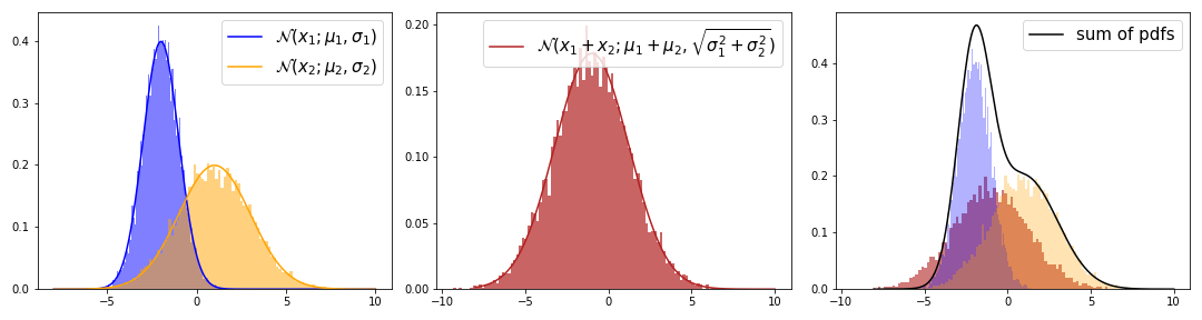
To understand why the red and black lines differ we will look at one particular way to derive the sum of RVs.
Let \(X_1\) and \(X_2\) be two independent RVs with pdfs \(f_1(X_1)\) and \(f_2(X_2)\). Then we can define a transformation \(g(x_1, x_2)\) mapping from \(X\) to a new random variable \(Y\) with
\[\begin{aligned} w_1 &= x_1 + x_2 \\ w_2 &= x_2 \end{aligned}\]and inverse transformation \(g^{-1}(w_1, w_2)\)
\[\begin{aligned} x_1 &= w - w_2 \\ x_2 &= w_2 \end{aligned}\]With the change of variable formula for probability densities we can compute the probability distribution of \(Y\) with
\[\begin{aligned} f_Y(w_1,w_2) &= f(g^{-1}(w_1,w_2)) \vert J \vert \\ &= f_1(w_1-w_2) f_2(w_2) \vert J \vert \\ \end{aligned}\]where \(\vert J \vert\) is the determinant of the Jacobian \(\left\vert \frac{\partial}{\partial y} g^{-1}(Y) \right\vert\), i.e.
\[\begin{aligned} J &= \left \vert \begin{pmatrix} \frac{\partial x_1}{\partial w_1} & \frac{\partial x_1}{\partial w_2} \\ \frac{\partial x_2}{\partial w_1} & \frac{\partial x_2}{\partial w_2} \end{pmatrix} \right \vert \\ &= \left \vert \begin{pmatrix} 1 & -1 \\ 0 & 1 \end{pmatrix} \right \vert = 1 \end{aligned}\]To get the distribution of \(w_1\) we have to marginalize out \(w_2\).
\[\begin{aligned} f(w) &= \int_{-\infty}^{+\infty} f_1(w_1 - w_2) f_2(w_2) dw_2 \\ \end{aligned}\]This describes the Convolution of two pdfs. The convolution of two Gaussian pdfs is another Gaussian pdf with parameters \(\mu = \mu_1 + \mu_2\) and \(\sigma^2 = \sigma_1^2 + \sigma_2^2\) (see e.g. this proof). We can visually confirm this result.
If you want to step through the GIF at your own pace you can find an HTML version in the GitHub repo (or show me how to embed HTML files in markdown). We can visually understand this derivation as well.
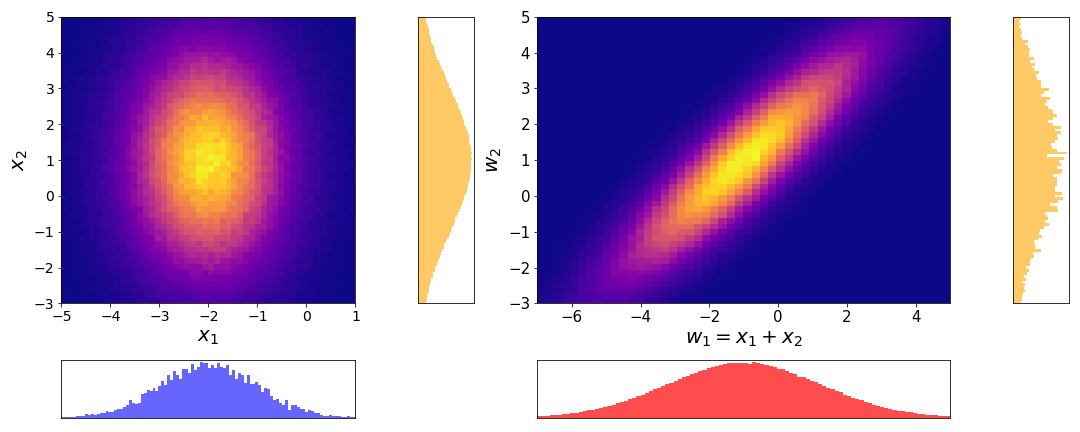
On the left we have the joint distribution \(p(x_1, x_2)\) of the two independent Gaussian RVs \(X_1\) and \(X_2\). Since they are independent, the joint is the same as the product of the marginals \(p(x_1, x_2) = p(x_1) \cdot p(x_2)\). The marginals are the same distributions as in the first figure of this chapter. On the right we have the joint distribution after the transformation \(p(w_1, w_2)\). We see that the marginal distribution \(p(w_1)\) is similar to the histogram of the sum of Gaussian random variables. This shows, that applying the change of variable formula and computing the marginal yields the correct distribution for \(X_1 + X_2\).
Now we understand better where the difference between the sum of RVs and the sum of pdfs comes from. The sum of RVs is an operation applied to the RVs themselves while the sum of pdfs is applied to a function of the RVs. When formulated as a function of pdfs, the sum of RVs turns out to be their convolution - which is clearly not the sum of pdfs.
Products
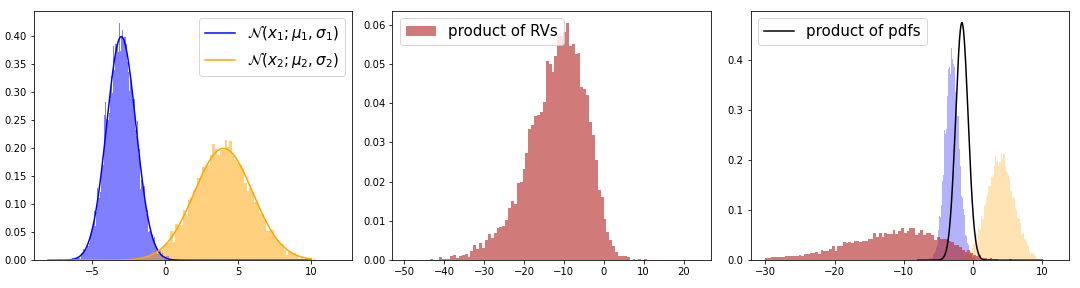
In general, the product of two RVs of the same distribution doesn’t have to follow this distribution. For example, the product of two Gaussian RVs is not a Gaussian. But the product of two Gaussian pdfs is proportional to a new Gaussian. The red and black distributions visualize this discrepancy.
To understand why this is the case, we once again look into how the product of RVs translates into a function of their pdfs. Similar to the case of the sum, we have independent RVs \(X_1, X_2\) with pdfs \(f_1(X_1)\) and \(f_2(X_2)\) and a transformation \(h(x_1, x_2)\) from \(X\) to \(Y\).
\[\begin{aligned} z_1 &= x_1 \cdot x_2 \\ z_2 &= x_2 \end{aligned}\]and inverse transformation \(h^{-1}(z_1, z_2)\)
\[\begin{aligned} x_1 &= z_1/z_2 \\ x_2 &= z_2 \end{aligned}\]Using the change of variable formula for pdfs we get the pdf of \(Y\).
\[\begin{aligned} f_Y(z_1,z_2) &= f(h^{-1}(z_1/z_2)) \vert J \vert \\ &= f_1(z_1/z_2) f_2(z_2) \vert J \vert \\ \end{aligned}\]with Jacobian
\[\begin{aligned} J &= \left \vert \begin{pmatrix} \frac{\partial x_1}{\partial z_1} & \frac{\partial x_1}{\partial z_2} \\ \frac{\partial x_2}{\partial z_1} & \frac{\partial x_2}{\partial z_2} \end{pmatrix} \right \vert \\ &= \left \vert \begin{pmatrix} \frac{1}{z_2} & -\frac{y}{x_2^2} \\ 0 & 1 \end{pmatrix} \right \vert = \vert \frac{1}{z_2} \vert \end{aligned}\]Inserting \(J\) and marginalizing out \(z_2\) we get
\[f(z_1) = \int_0^{+\infty} \frac{1}{z_2} f_1\left(\frac{z_1}{z_2}\right) f_2(z_2) dz_2\]which is known as the Mellin convolution of \(f_1(x_1)\) and \(f_2(x_2)\).
If you want to step through the GIF at your own pace you can find an HTML version in the GitHub repo. The derivation through the joint can be understood visually as well.
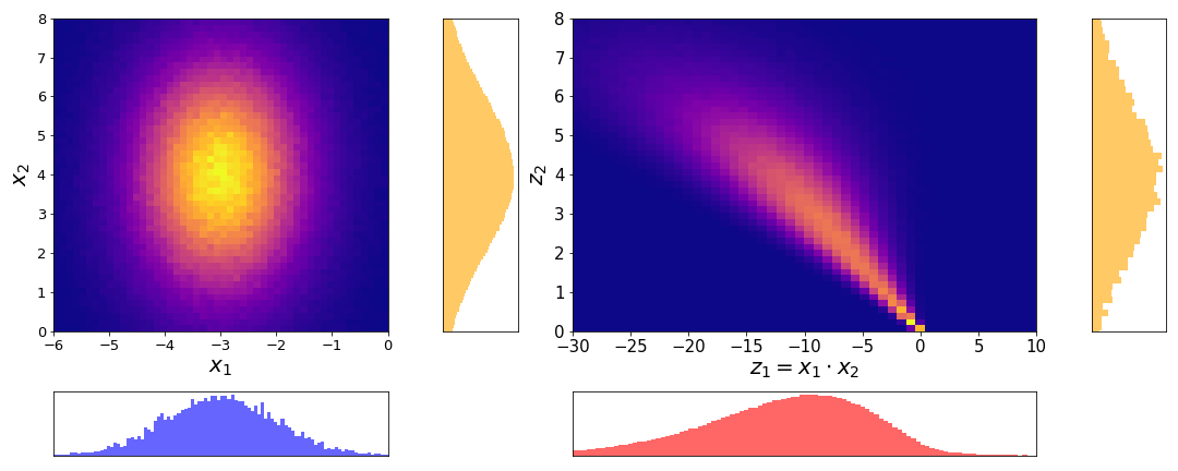
On the left we have the joint distribution \(p(x_1, x_2)\) of the two independent Gaussian RVs \(X_1\) and \(X_2\) with respective marginal distributions. On the right we have the joint distribution after the transformation \(p(z_1, z_2)\). We see that the marginal distribution \(p(z)\) is similar to the histogram of the product of Gaussian RVs from the first figure of this chapter.
Similar to the case of the sum, we can now clearly see that the product of two independent RVs does not translate to the product of their pdfs, but rather to their Mellin.
Examples
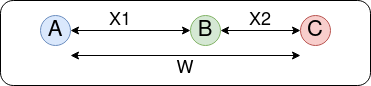
Sum: Assume there are three houses - yours \((A)\), your mom’s \((B)\) and your grandpa’s \((C)\). The path from your house to your grandpa’s goes past your mom’s house. You measure the distance \(X_1\) from \(A\) to \(B\) and your mom measures the distance \(X_2\) from \(B\) to \(C\) but you are ultimately interested in the distance from \(A\) to \(C\), \(W=X_1 + X_2\). Your measurement is noisy, e.g. because you estimate the distance y counting the number of steps. Thus \(X_1, X_2\) and \(W\) are random variables. If the noise of your measurement is Gaussian then the sum of the measurements \(W\) is distributed according to a Gaussian again. The sum of pdfs \(p_1(x_1) + p_2(x_2)\) doesn’t have any real-life interpretation that I would be aware of.
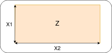
Product: Assume you own a rectangular piece of land and want to estimate its area. You measure the length of one side \(X_1\) and the other \(X_2\). Once again, we assume a Gaussian measurement error. Then the random variable describing the area \(Z = X_1 \cdot X_2\) is not distributed according to a Gaussian. The product of the pdfs, \(p_1(x_1) \cdot p_2(x_2)\), is proportional to a Gaussian but has no relation to the area. It can be interpreted as the likelihood of \(X_1\) and \(X_2\). With the likelihood, we can determine how likely a given combination of observed measurement values \(x_1, x_2\) are under the assumption of Gaussian measurement noise.
Conclusion
Applying an operation to an RV yields a different distribution than applying the same operation to their pdfs. Using the derivations above, we found that the pdf for the result of an operation on RVs can be computed through a change of variables and marginalization. In the cases of independent RVs, the pdfs for sums and products are described by different forms of convolutions. Since convolution is neither equivalent to the sum nor the product of the RVs, we now understand why they yield different results.
If you have a practical application and don’t know which of the two to apply you can think about whether you apply a given operation to a random variable or to their probability density function. For example, the sum of eyes of two dice is an operation that acts on the random variable itself. Bayes rule, on the other hand, describes a product of the probabilities of random variables and is thus an operation between pdfs.
If you want to understand the math more rigorously, I can recommend The Algebra of Random Variables. Even though the book has been published in 1979 already, it still contains all relevant derivations and is easy to read.
One last note
If you want to get informed about new posts you can subscribe to my mailing list or follow me on Twitter.
If you have any feedback regarding anything (i.e. layout or opinions) please tell me in a constructive manner via your preferred means of communication.