What is this post about?
Exponential family distributions are important for many classical machine learning applications. Their properties form the basis of Expectation Propagation and they are often used in hierarchical probabilistic models. Because of this, they are well-documented and many tutorials exist. Most resources on exponential families are rather math-heavy and some people learn best with this approach. However, I personally think and learn primarily in a visual fashion and many others do too. Thus I want to provide a tutorial on exponential families and some of their properties with a focus on visual interpretations whenever possible.
The Basics
A pdf that can be written in the form
\[\begin{aligned}\label{EF} p(x) &= h(x)\cdot \exp\left(w^\top \phi(x) - \log Z(w) \right) \end{aligned}\]where
\[\begin{aligned} Z(w)&:= \int_{\mathbf{X}} h(x)\exp\left(w^\top \phi(x)\right) \,dx \end{aligned}\]is called an exponential family. \(\phi(x): \mathbb{X} \rightarrow \mathbb{R}^d\) are the sufficient statistics, \(w \in \mathcal{D} \subseteq \mathbb{R}^d\) the natural parameters with domain \(\mathcal{D}\), \(\log Z(w): \mathbb{R}^d \rightarrow \mathbb{R}\) is the (log) partition function (normalization constant), and \(h(x): \mathbb{X} \rightarrow \mathbb{R}_{+}\) the base measure.
Many distributions can be written as exponential families (see e.g. Wikipedia). Some of the most prominent ones are the Normal, Beta, and Gamma distribution which are displayed for three sets of parameters respectively.
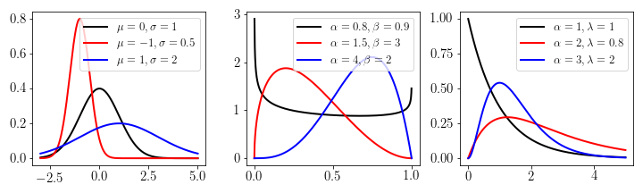
To show how an exponential family distribution is transformed from standard form to exponential family form, consider the example of the Beta distribution.
\[\begin{aligned} \mathcal{B}(x, \alpha, \beta) &= \frac{x^{(\alpha - 1)} \cdot (1-x)^{(\beta-1)}}{B(\alpha, \beta)} \\ &= \exp\left[(\alpha-1) \log(x) + (\beta-1)\log(1-x) - \log(B(\alpha,\beta)))\right]\\ &= \frac{1}{x(1-x)}\exp\left[\alpha\log(x) + \beta\log(1-x) - \log(B(\alpha,\beta)))\right] \end{aligned}\]with exponential family values \(h(x) = \frac{1}{x(1-x)}, \phi(x)=(\log(x), \log(1-x)), w = (\alpha, \beta)\) and \(Z(\alpha, \beta) = \log(B(\alpha,\beta))\) where \(B(\alpha, \beta) = \frac{\Gamma(\alpha)\Gamma(\beta)}{\Gamma(\alpha + \beta)}\) and \(\Gamma(x)\) is the Gamma function.
The sufficient statistics are the statistics of the data that tell you everything interesting about them, i.e. if you know the sufficient statistics another person with the same data is unable to tell more about the probability distribution than you are. For the normal distribution, for example, the sufficient statistics are \(Y_1 = \sum_i X_i\) and \(Y_2 = \sum_i X_i^2\) for samples \(X_i, i=1,...,N\). With \(Y_1\) and \(Y_2\) we can compute
\[\begin{aligned} M &= 1/n Y_1 \\ S^2 &= \frac{Y_2 - (Y_1^2/n)}{n-1} \\ &= \frac{1}{n-1} \left[\sum_i X_i^2 - n\overline{X}^2\right] \end{aligned}\]to rediscover the mean and standard deviation which are also sufficient estimators of the normal distribution.
The natural parameters are the set of parameters \(w\) for which \(p(x)\) is defined. They are related to (but usually not the same as) the parameters of the probability distribution. The parameters of the normal distribution, for example, are its mean \(\mu\) and standard deviation \(\sigma\). Its natural parameters, however, are \(w_1 = \frac{\mu}{\sigma^2}\) and \(w_2 = -\frac{1}{2\sigma^2}\).
The base measure is the fuzziest part of exponential families in my experience. This is because we can arbitrarily shift values between the natural parameters and the base measure. The following three equations, for example, are all possible legitimate definitions of the Beta distribution in exponential family form but they have different base measures and natural parameters.
\[\begin{aligned} \mathcal{B}(x, \alpha, \beta) &= 1 \cdot \exp\left[(\alpha-1)\log(x) + (\beta-1)\log(1-x) - \log B(\alpha, \beta) \right] \\ &= \frac{1}{x(x-1)} \exp\left[(\alpha)\log(x) + (\beta)\log(1-x) - \log B(\alpha, \beta) \right] \\ &= \frac{1}{x^2(x-1)^2} \exp\left[(\alpha+1)\log(x) + (\beta+1)\log(1-x) - \log B(\alpha, \beta) \right] \end{aligned}\]However, the most reasonable definition is one where we push all “left-over” parts from the natural parameters into the base measure, e.g. the \(-1\) terms in the Beta distribution (see second equation above). The reason why it is called “base-measure” is that if you set your natural parameters \(w\) to 0, only your base is left. Similarly, you could say that changing your natural parameters \(w\) can be seen as updating your base measure \(h(x)\).
The log partition function: is the most underrated part of exponential families. In the beginning, I perceived it as “just a normalizing constant” to ensure that the distribution integrates to one. However, the fact that it is available in closed form combined with the structure of exponential families yields very powerful properties. I will discuss them further down in more detail but, in short, the log partition function allows for efficient computation of the moments through derivation instead of integration. This is powerful because derivation is usually much easier than integration.
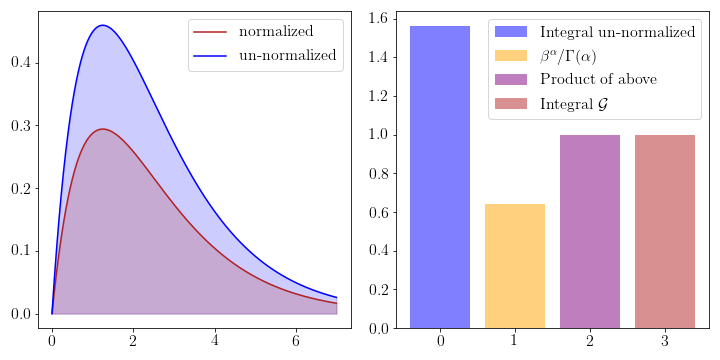
To understand the normalizing effect of the log partition function consider the following figure where the Gamma distribution has been plotted with and without the normalizing constant.
If you want to find the natural parameters \(w\), sufficient statistics \(\phi(x)\), base-measure \(h(x)\) or log partition function \(\log Z(w)\) and don’t want to calculate them by hand, you can find a large table of them on Wikipedia.
Important Properties
Exponential Families have a lot of interesting properties. I chose a small selection of the ones I find most important. Since I come from a Machine Learning background, my selection is biased towards ML.
Multiplication and Division
Due to the properties of the exponential function, the product and division of exponential family PDFs is proportional to another instance of the same exponential family. Assume we have an exponential family with two different parameterizations \(w_1\) and \(w_2\). Then we can write
\[\begin{aligned} p_1(x) \cdot p_2(x) &= h(x)\cdot \exp\left(w_1^\top \phi(x) - \log Z(w_1) \right) \cdot h(x)\cdot \exp\left(w_2^\top \phi(x) - \log Z(w_2) \right) \\ &= \frac{1}{Z(w_1)} \exp((w_1 + c) \phi(x)) \cdot \frac{1}{Z(w_2)} \exp((w_2 + c) \phi(x)) \\ &= \frac{1}{Z'} \exp((w' + c') \phi(x)) \\ &\propto \frac{1}{Z} h(x) \cdot \exp((w') \phi(x)) \\ \end{aligned}\]which is again in the form of the same exponential family. I use \(h(x)\) and \(c\) interchangeable, since multiplying with the base measure is similar to adding a constant to the natural parameters (see section on base measure above). A similar result can be derived for division just that \(w' = w_1 - w_2\) instead of \(w' = w_1 + w_2\). Of course, the \(w'\) have to be valid parameters, e.g. the variance of a Gaussian cannot be negative. To see this property visually for the Beta and Normal distribution consider the following figure.
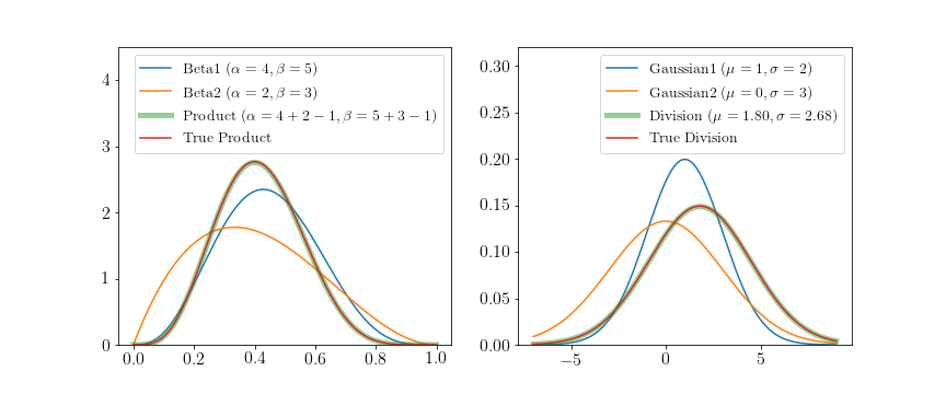
The true distributions have been computed by multiplying/dividing distribution 1 and 2 and re-normalizing the results. The update rule for the Beta distribution is simply \(\alpha' = \alpha_1 + \alpha_2 -1, \beta' = \beta_1 + \beta_2 - 1\) and for the Gaussian distribution
\(\mu' = \frac{\mu_1 \sigma_2^2 - \mu_2 \sigma_1^2}{\sigma_1^2 + \sigma_2^2}\) and \(\sigma' = \sqrt{\frac{1}{\frac{1}{\sigma_1^2} - \frac{1}{\sigma_2^2}}}\).
While this looks like an insignificant property it is actually very important. It implies that we can update the parameters of distributions by simple addition instead of computing costly approximations. This property is a key component of the Machine Learning technique Expectation Propagation.
Conjugacy
Bayesian Inference is done via Bayes Theorem
\[p(\theta \vert X) = \frac{p(X \vert \theta) p(\theta)}{p(X)} = \frac{p(X \vert \theta) p(\theta)}{\int p(X \vert \theta) p(\theta)}\]Where \(p(\theta \vert X)\) is called posterior, \(p(X \vert \theta)\) likelihood, \(p(\theta)\) prior, and \(\int p(X \vert \theta) p(\theta)\) evidence. In general, the product of two probability distributions does not yield a new probability distribution in closed-form. Therefore, we have to apply approximations or costly sampling strategies to get the posterior probability density. However, when the prior distribution is conjugate to the likelihood, the posterior is of the same form as the prior and its parameters can be updated in closed-form. This comes as a blessing since it removes all of the complexity of Bayesian inference. Most distributions are not conjugate with each other but for commonly used likelihoods, there exists an exponential family conjugate prior. A Bernoulli likelihood, for example, has a Beta conjugate prior.
I think conjugacy can be easiest understood in visual terms. Thus, in the following, you can see how different data types update their respective conjugate priors. The figures on the left contain the conjugate distribution and the figure on the right is used to generate the data.
If you find the speed of the GIF too high or low or want to pause it at some point you can always just pull the github repo and step through the HTML files at your own pace.
Beta
The Beta distribution describes beliefs about a probability, thus it is plausibly the conjugate prior to Bernoulli and Binomial likelihoods. In both cases we start with a flat Beta prior, i.e. \(\alpha=\beta=1\). On the right-hand side, the distributions of the likelihood are shown in blue and the samples that simulate the data are drawn in black. Per step, we draw one sample and update our current Beta distribution accordingly.
For the Bernoulli likelihood this means we compute \(\alpha' = \alpha + \sum_i x_i\) and \(\beta' = \beta + n - \sum_i x_i\), i.e. we add 1 to \(\alpha\) for every success and 1 to \(\beta\) for every failure.
For the Binomial likelihood we compute \(\alpha' = \alpha + \sum_i x_i\) and \(\beta' = \beta + \sum_i N_i - \sum_i x_i\).
The posterior updates have a very intuitive interpretation. If we have more data, the Beta mean gets closer to the true probability and its uncertainty decreases. The more coinflips we see the better we know its bias and the more certain we become.
Mean of a Normal (with known variance)
The conjugate prior for the mean of a Gaussian (not the entire Gaussian distribution) is a Gaussian. In other words, the more data points you have from a Gaussian distribution the more certain you are about its mean. The update equations for this setup are
\[\begin{aligned} v' &= \frac{1}{\frac{1}{\sigma_0^2} + \frac{n}{\sigma^2}} \\ m' &= v' \cdot \left(\frac{\mu_0}{\sigma_0^2} + \frac{\sum_i x_i}{\sigma^2} \right) \end{aligned}\]
Our goal is to estimate the mean of the Gaussian distribution on the right, i.e. the red line. In the beginning, we have no clue about its position and start with a standard normal prior (blue line on the left). The more samples (black) we see from the true distribution, the more our posterior estimate for the mean (red line on the left) gets closer to the true mean and its variance decreases.
Gamma
The Gamma is a distribution over positive quantities. It is a conjugate prior to the rate parameter of Poisson likelihoods, which are discrete distributions over rare events, e.g. earthquakes. So if you have count data of earthquakes and you assume them to be generated by a Poisson distribution you can get a posterior distribution over its rate parameter with
\(\alpha' = \alpha + \sum_i x_i\) and \(\beta' = \beta + n\)
We find that with more data the posterior distribution over the \(\lambda\) rate parameter gets closer to the true value of 0.5 and the uncertainty decreases.
Dirichlet
Similar to how the Beta distribution describes believes about one probability, the Dirichlet describes beliefs about a probability vector. It is a conjugate prior to categorical and multinomial likelihoods. Let’s say, for example, we have three categories (or types) of texts: politics, finance, and sports and we read a newspaper containing three texts every day (they can contain multiple texts of the same type). Then we might be interested in which kind of focus the publisher has, i.e. what the generating distribution for the texts is. Every individual newspaper can be modeled by a Binomial distribution with \(n=3\). The generating can be modelled by a Dirichlet and updated with \(\alpha' = \alpha + \sum_i x_i\).
We can see that the mean of the posterior Dirichlet function gets ever closer to the true probabilities generating the Binomial likelihoods and that the uncertainty of our estimate decreases. In our metaphor, this means that after seeing many individual newspapers we think that the outlet focuses mostly on politics (60%), a bit on finance (25%), and even less on sports (15%).
Inverse Wishart
The inverse Wishart is a distribution over symmetric positive semi-definite matrices. It is a conjugate prior to empirical covariance matrices, e.g. the outer product of vectors drawn from a zero-mean Gaussian. I always found it hard to get a good grasp of the inverse Wishart distribution and thus first want to introduce it in slightly more detail than the other distributions.
First of all, the inverse Wishart (and the Wishart) distribution is defined on the symmetric positive semi-definite (psd) cone. The psd cone is a subspace of \(\mathbb{R}^d\) on which all psd matrices lie. A real symmetric matrix \(\begin{pmatrix} a & b \\ b & c \end{pmatrix}\) is psd iff \(a, c \geq 0\) and \(ac - b^2 \geq 0\). Following this stackoverflow post, we will represent this by \((a, b, c) \in \mathbb{R}^3\). If we set \(a=1\) then \(c \geq b^2\) and if we set \(c=1\) then \(a \geq b^2\). So if we plot \((a,b,c) = (1, b, b^2)\) and \((a,b,c) = (b^2, b, 1)\) for \(-1 \leq b \leq 1\) respectively and join these points with \((0,0,0)\) we start to see the cone.
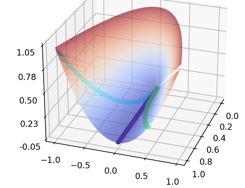
If you want to view the cone from different angles you can do so in the respective jupyter notebook.
It is very hard to plot the density of a probability distribution on this cone. Thus we have to fall back on other strategies to plot the inverse Wishart distribution. I will use two different tools to plot the Wishart distribution.
The first requires a bit of math. For off-diagonal elements of a symmetric psd matrix \(A\) it holds \(a_{ij}^2 \leq a_{ii} a_{jj}\) (see e.g. here). Thus for our 2-dimensional case we know that \(b = \rho \cdot \sqrt{ac}\) for \(\rho \in (-1, 1)\). So one way to visualize the Wishart is to plot marginals for different values of \(\rho\) with increasing \(a\) and \(c\). The green, purple and blue line in the above plot show the locations of the marginals for \(\rho\) equal to \(0.5, 0\) and \(-0.99\) respectively.
Computing the pdf of the inverse Wishart for \(\rho = -0.9,-0.8,...,0.8,0.9\) from most blue to most red results in the following figure.
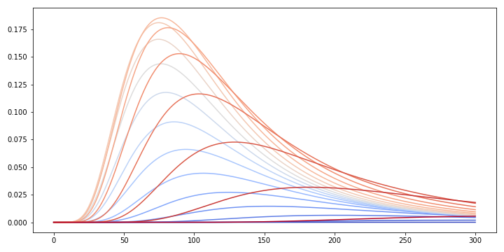
The scale-matrix \(\Psi\) for this figure is \(\begin{pmatrix} 5 & 1 \\ 1 & 2 \end{pmatrix}\). Since the off-diagonal elements are positive, the probability mass is larger for positive values of \(\rho\) (red curves) than for negative values (blue curves).
The second tool is simpler. It shows histograms of \(a, b\) and \(c\) for samples drawn from the (inverse-) Wishart.
To visualize the likelihood we draw samples from a 2-dimensional Gaussian (top right) and compute their outer products. The update rules for the inverse Wishart are \(\Psi' = \Psi + \sum_i x_i x_i^\top\) and \(\nu' = \nu + n\).
Combining all this we can inspect how the Wishart distribution behaves when updated with Gaussian outer product likelihoods.
In our first visualization (top left) we find that a) similar to the one-dimensional cases, the probability distribution “wanders” to the true solution. Remember that the figure displays marginals and the curves thus do not integrate to one. b) The off-diagonal entries of \(\Psi\) are both 0 in the prior and thus \(-\rho\) and \(+\rho\) yield the same marginal distribution. With every update, the off-diagonal values of \(\Psi\) get more positive and thus \(-\rho\) and \(+\rho\) yield different marginal distributions. Thus, the larger the off-diagonal entries of \(\Psi\) become, the more probability mass is with the red curves while the blue curves vanish.
In the second visualization (bottom) we find that the histograms of \(a, b\) and \(c\) for 1000 samples of the Wishart get narrower over time. This shows how the uncertainty decreases and we get more and more certain about the underlying psd matrix.
Overall, I find it hard to think about or explain the inverse Wishart distribution because high-dimensional objects in general – and especially on the psd cone – are hard to visualize.
Moment calculation
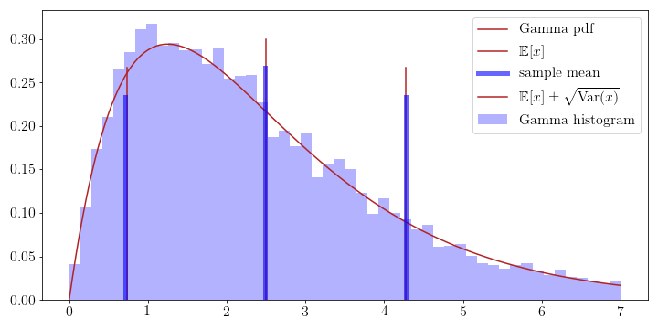
The moments of exponential families can be computed by differentiating the log-partition function. In this section, I want to show why this is possible and derive the mean and variance for the Gamma distribution.
In general, the moment-generating function (MGF) of a random variable \(X\) is
\[M_X(t) := \mathbb{E}\left[e^{tX} \right], \qquad t \in \mathbb{R}\]wherever this expectation exists. \(M_X(0)\) always exist and is 1, since probability density functions have to integrate to 1. The cumulant-generating function CGF is defined as the logarithm of the MGF
\[K(t) = \log \mathbb{E} \left[e^{tX} \right], \qquad t \in \mathbb{R}\]For exponential families, this means that the MGF of the sufficient statistics \(\phi(x)\) is
\[M_{\phi(x)}(u) = \mathbb{E}[e^{u^\top \phi(x)} | w] = \int_x h(x) \exp((w+u)^\top \phi(x) - Z(w)) dx = \exp(Z(w + u) - Z(w))\]which means that the CGF is
\[K_{\phi(x)}(u) = Z(w + u) - Z(w)\]which is obviously not \(Z(w)\). However, if we take derivatives of \(K(u)\) w.r.t. \(u\) and then set \(u\) equal to zero (to obtain the coefficients of the Taylor-series expansion), we get the same answer as is obtained by taking derivatives of \(Z(w)\) w.r.t. \(w\).
In general, the cumulants are not similar to the central moments of a probability distribution. However, the mean, variance, and third central moment are identical and for the rest of this tutorial, we only care about the first and second central moments.
To illustrate this further, we derive the mean and variance of the Gamma distribution (the same derivation can also be found on Wikipedia). The pdf of the Gamma distribution is
\[p(x) = \frac{\beta^\alpha}{\Gamma(\alpha)} x^{\alpha-1} e^{-\beta x}\]and its natural parameters are \(w_1 = \alpha-1\) and \(w_2 = -\beta\). Their reverse substitutions are \(\alpha = w_1 + 1\) and \(\beta = -w_2\). The sufficient statistics are \((\log x, x)\) and the log-partition function as a function of the natural parameters is
\[Z(w_1, w_2) = \log \Gamma(w_1 + 1) - (w_1 + 1) \log(-w_2)\]To compute the mean we need to differentiate the log-partition function w.r.t. \(w_2\) since the second sufficient statistic is \(x\). Thus
\[\begin{aligned} \mathbb{E}[x] &= \frac{\partial Z(w_1, w_2)}{\partial w_2} \\ &= -(w_1 + 1)\frac{1}{-w_2}(-1) = \frac{w_1 + 1}{-w_2} \\ &= \frac{\alpha}{\beta} \end{aligned}\]To compute the variance we differentiate twice and get
\[\begin{aligned} \mathrm{Var}(x) &= \frac{\partial^2 Z(w_1, w_2)}{\partial w_2} \\ &= \frac{\partial}{\partial w_2} \frac{w_1 + 1}{-w_2} \\ &= \frac{\alpha}{\beta^2} \end{aligned}\]We can visually confirm, that these approximations are correct by comparing sampling-based and closed-form solutions.
Similar to above we can also compute the moments for the other sufficient statistics, e.g. \(\mathbb{E}[\log x]\) and \(\mathrm{Var}(\log x)\).
All of the moments above can also be computed using integration but it is significantly more complicated than differentiation.
Moment Matching
Let’s say we have two distributions \(p(x)\) and \(q(x)\) where \(p\) is any fixed distribution and \(q\) is a member of an exponential family. Then we can show that the KL-divergence \(KL(p\vert\vert q)\) between the two distributions is minimized by matching their moments, e.g. setting the mean and variance of \(p(x)\) to that of \(q(x)\). We write
\[\begin{aligned} KL(p||q) &= \int p(x) \log\frac{p(x)}{q(x)} dx \\ &= \int p(x) \log p(x) dx - \int p(x) \log q(x) dx \\ &= \mathbb{E}_{p(x)}[\log p(x)] - \int p(x) \log\exp(w \phi(x) + \log h(x) - \log Z(w)) dx \\ &= \mathbb{E}_{p(x)}[\log p(x)] - \mathbb{E}_{p(x)}[\log h(x)] - \mathbb{E}_{p(x)}[w \phi(x)] + \mathbb{E}_{p(x)}[\log Z(w)] \end{aligned}\]which as a function of \(w\) is
\[KL_w(p||q) = - \mathbb{E}_{p(x)}[w \phi(x)] + \log Z(w)\]where the expectation around \(\log Z(w)\) vanishes as it is independent of \(x\). To get the optimal values for \(w\) we compute the first derivative w.r.t. \(w\) and set it to zero.
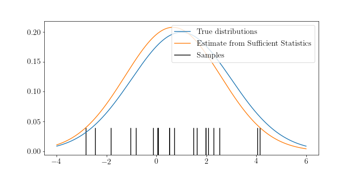
\[\begin{aligned} \nabla_w KL_w(p||q) &= - \mathbb{E}_{p(x)}[\phi(x)] + \nabla_w \log Z(w) \overset{!}{=} 0 \\ \Leftrightarrow \nabla_w \log Z(w) &= \mathbb{E}_{p(x)}[\phi(x)] \\ \Leftrightarrow \mathbb{E}_{q(x)}[\phi(x)] &= \mathbb{E}_{p(x)}[\phi(x)] \end{aligned}\]where we use the knowledge that the derivatives of the log-partition function yield the moments of the distribution which we derived in the previous section. The visual intuition behind this fact can be found in the figure below. Our static distribution \(p(x)\) is a normal with \(\mu=4\) and \(\sigma=1\) and we want to fit a Gamma distribution \(q(x)\) such that \(KL(p\vert\vert q)\) is minimized. To match the moments we compute
\[\begin{aligned} \mu &= \frac{\alpha}{\beta} \\ \sigma^2 &= \frac{\alpha}{\beta^2} \\ \Rightarrow \alpha &= \frac{\mu^2}{\sigma^2} = 16\\ \Rightarrow \beta &= \frac{\mu}{\sigma^2} = 4 \end{aligned}\]We can then compare the empirical KL divergences for different pairs of parameters around the theoretically optimal solution to convince ourselves that we have the best fit.
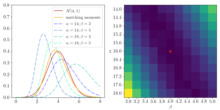
This property of matching the moments (or expectations) gives name to Expectation Propagation since one of its central steps is to fit an exponential family by moment matching.
Conclusion
When I first learned of exponential families I thought “It’s just a different way to write probability densities, why does it matter?”. But after working with and reading about their properties for about a year now, I learned that they are much more powerful. Exponential families have conjugate priors and thus we can compute posteriors in closed form. This is a huge benefit over sampling-based approaches such as MCMC. Furthermore, exponential families are “closed” under multiplication and division which - once again - implies fast computations. Their normalizing constants (the log-partition function) are available in closed-form. Therefore we can compute their moments through differentiation instead of integration saving us a lot of pain. On a related note, we can show that the KL-divergence between two exponential families is minimized by matching their moments. Overall, a seemingly simple way to write different probability density functions has pretty large implications and yield the foundations of different algorithms for Bayesian generalized linear models (GLMs), Expectation Propagation, and many more.
My own research is closely linked to exponential families. Maybe you are interested in
- A cool trick in Bayesian neural networks [blog] [arxiv]
- A new technique to make GLMs really fast [soon]
- My current research project [will take a while]
One last note
If you want to get informed about new posts you can subscribe to my mailing list or follow me on Twitter.
If you have any feedback regarding anything (i.e. layout or content) please tell me in a constructive manner via your preferred means of communication.