Update
When I wrote this post, the paper was not published yet. Now, after multiple resubmissions it has been accepted to UAI2022. Since we changed some substantial parts of the paper during the resubmissions, I decided to rewrite and update this post. The original post was published on the 3rd of November 2020.
My personal opinion
The idea underlying the Laplace Bridge for BNNs is very clean–you take a slow part in a Bayesian Neural Network and replace it with a fast approximation. However, the longer I worked with the LB, the more I realized that the approximation just isn’t that good. It has some theoretical problems but more importantly it is very easy to create examples with bad approximation quality. We could fix some of these problems with correction terms but even then the approximation quality of the LB is bad for some relevant cases.
Therefore, the main reasons to care about the LB are: a) when inference speed matters much more than accuracy, e.g. when you just need some uncertainty estimate very quickly. Since drawing samples has gotten quite faster, I think there is basically nearly no practical use-case for the LB. b) A thought provoking way to think about BNNs. Working with the LB mostly showed me that there are many ways to achieve predictive uncertainty and we have probably only scratched the surface.
Unfortunately, the current publishing environment doesn’t allow me to write papers in which I can express my opinion as honest as here. But on my blog I can say whatever I want and I think it’s important for other researchers to get my honest view. In all likelihood, you shouldn’t think about the LB for BNNs or use it in practice unless you are in one of the rare use-cases described above. Save yourself the time and work on something more promising.
What is the paper about?
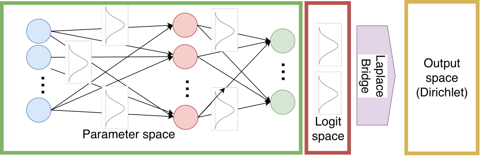
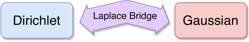
Bayesian inference in Neural Networks is typically very costly. However, it is often desirable because it yields distributions as outputs instead of just point estimates. This paper takes one step in the direction of making Bayesian inference faster by speeding up one part of the pipeline significantly. In the following figure, you can see that we approximate the output distribution with a Dirichlet via the Laplace Bridge instead of sampling from the distribution of logits and applying the softmax function.
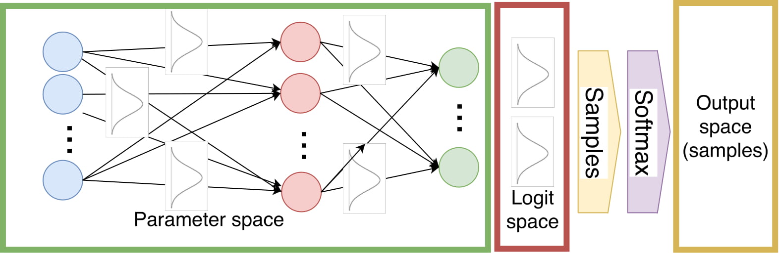
While this might look like a small change it turns out to be a pretty drastic speed up and has a non-negligible effect on the overall prediction time while providing estimates of similar quality. Additionally, it yields a fully parameterized distribution instead of just samples.
The paper can be found on arxiv. The accompanying code is available on GitHub
Motivation
Neural Networks usually yield point estimates as outputs. An image classifier might, for example, classify an image as a dog with 75 percent probability. However, it does not give us an estimate of the uncertainty which is attached to this estimate. The network could either be very certain that this is an image that warrants a 75 percent probability for the class dog or it could be like “meh, I don’t know, probably a dog” or anything in between. Especially in safety-critical applications, this notion of uncertainty becomes more relevant. If you want a network to detect cancer you might also be interested in the uncertainty of your estimate. If, for example, the network estimates the probability for skin cancer lower than for no skin cancer but has high uncertainty you might want a human to double-check the images to make sure the detection worked correctly. Similarly, in a self-driving car, you might want to have certain safety mechanisms when the classification for pedestrians has high uncertainty even when the expected value of the estimate is high.
Unfortunately though getting these distributions is usually associated with high computational costs. Either expensive operations have to be performed, such as the computation of the Hessian or any of its many approximations, or samples have to be drawn from different parts of the network pipeline. The Laplace Bridge (LB) for Bayesian Neural Networks (BNN) avoids the sampling process by providing a closed-form approximation of the posterior distribution and thereby speeds up a relevant part of the prediction process. This is especially helpful in applications where speed makes an important difference such as self-driving cars.
Theory
Before we get into the details of its application to BNNs we first have to understand the Laplace Bridge
The Laplace Bridge
Two pieces of background information are important to understand the LB.
Change of Variable for PDFs: Every probability distribution \(p(x)\) can be represented in a different base \(y\) by transforming its variable with \(g(x)\) and multiplying it with the Jacobian of the inverse transformation to ensure that the distribution still integrates to 1. In equations this means
\[p_y(y) = p_x(g^{-1}(x)) \det\left(\frac{\partial g^{-1}(x)}{\partial y}\right)\]For a simplified intuition you can think of the change of variable as stretching or shrinking the distribution in a potentially non-linear way. I have written a more detailed explanation of change of variables here.
Laplace Approximation: A common way to approximate a function with a normal distribution is by using a Laplace approximation. This is done by using the mode of the function as the mean of the Normal \(\mu =\)argmax\(_x p(x)\) and the covariance matrix as the invere Hessian \(\Sigma = \frac{\partial^2 f(x)}{\partial^2 x}\). If \(\hat{\theta}\) denotes the mode of a pdf \(h(\theta)\), then it is also the mode of the log-pdf \(q(\theta) = \log h(\theta)\) since the logarithm is a monotone transformation. The 2-term Taylor expansion of \(q(\theta)\) is:
\[\begin{align} q(\theta) &\approx q(\hat{\theta}) + \nabla q(\hat{\theta})(\theta - \hat{\theta}) + \frac{1}{2}(\theta- \hat{\theta})\nabla\nabla q(\hat{\theta}) (\theta - \hat{\theta})\\ &= q(\hat{\theta}) + 0 + \frac{1}{2}(\theta- \hat{\theta})\nabla\nabla q(\hat{\theta}) (\theta - \hat{\theta}) \qquad \text{[since } \nabla q(\theta) = 0]\\ &= c - \frac{1}{2} (\theta - \mu)^\top \Sigma^{-1} (\theta - \mu) \end{align}\]where \(c\) is a constant, \(\mu = \hat{\theta}\) and \(\Sigma = \{-\nabla \nabla q(\hat{\theta})\}^{-1}\). The right hand side of the last line matches the log-pdf of a Gaussian. Therefore the pdf \(h(\theta)\) is approximated by the pdf of the normal distribution \(\mathcal{N}(\mu, \Sigma)\) where \(\mu = \hat{\theta}\) and \(\Sigma = \{-\nabla\nabla q(\hat{\theta})\}^{-1}\).
The last observation on our way to the Laplace Bridge is that a Dirichlet Distribution looks very much like a Gaussian when you change its variable via the softmax transformation \(\pi(x) = \frac{\exp(x_i)}{\sum_j \exp(x_j)}\). This can be seen visually in the following figure which contains the one-dimensional special case of the Dirichlet, the Beta distribution. We compare the Dirichlet in the standard base (left) and in the softmax base after applying the change of variable (right).
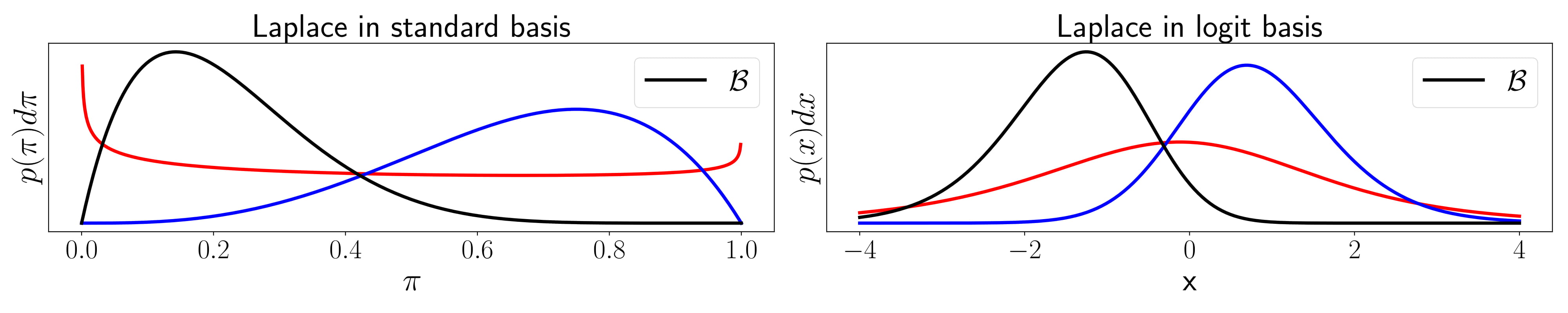
It is already visible that the Dirichlet in the softmax base looks significantly more like a Gaussian than in the standard basis. Now, we can apply a Laplace approximation in both bases to fit a Gaussian to the distribution. We can additionally transform the Gaussian from the Laplace approximation in the softmax basis back to the standard basis (right) and find that it is a better fit than the Laplace approximation in the standard base (left).
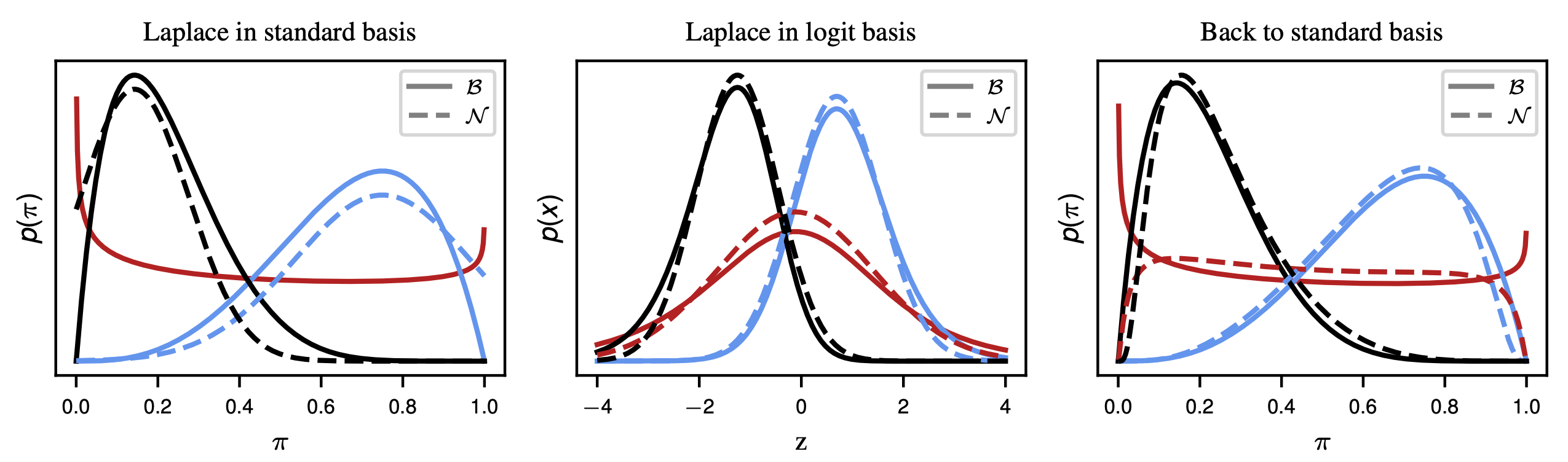
Furthermore, the Laplace approximation in the standard base is not always possible. When the Beta distribution encounters parameters that are smaller or equal to 1 it doesn’t have a well-defined mode anymore and a Gaussian can’t be fit (see the red line in the left figure). However, the same function with the same parameters can be fit in the softmax basis and this fit can also be transformed back to the original base (see red line in middle and right figure).
The change of basis is done by chosing \(g^{-1}(x)\) as the softmax function
\[\pi_k(\mathbf{z}) := \frac{\exp(z_k)}{\sum_{l=1}^K \exp(z_l)}\]such that the Dirichlet distribution
\[\mathrm{Dir}(\pi | \alpha) := \frac{1}{B(\alpha)}\prod_{k=1}^K \pi_k^{\alpha_k-1}\]becomes
\[\mathrm{Dir}_{z}(\pi(z) | \alpha) := \frac{1}{B(\alpha)}\prod_{k=1}^K \pi_k(z)^{\alpha_k}\]Applying a Laplace approximation in the softmax basis yields a direct map from \(\alpha\) to \(\mu\) and \(\Sigma\) which has already been derived by David J. MacKay in 1998.
\[\alpha_k = \frac{1}{\Sigma_{kk}}\left(1 - \frac{2}{K} + \frac{e^{\mu_k}}{K^2}\sum_l^K e^{-\mu_l} \right)\]My supervisor, Philipp Hennig, has derived the inverse mapping from \(\mu\) and \(\Sigma\) to \(\alpha\) during their Ph.D. under MacKay in 2010.
\[\mu_k = \log \alpha_k - \frac{1}{K} \sum_{l=1}^{K} \log \alpha_l\] \[\Sigma_{kl} = \delta_{kl} \frac{1}{\alpha_k} - \frac{1}{K} \left[\frac{1}{\alpha_k} + \frac{1}{\alpha_l} - \frac{1}{K} \sum_{u=1}^{K} \frac{1}{\alpha_u}\right]\]In summary, we have a fast, closed-form transformation between the parameters of a Dirichlet and a Gaussian
Lastly, I want to present a sanity check for the LB and its application to BNNs. In the following figure you can see five different scenarios of 3-dimensional Gaussians mapped through the Laplace Bridge. In the upper row are samples drawn from the Gaussian to which the softmax was applied. In the bottom row the values of the original Gaussian are mapped by the LB.
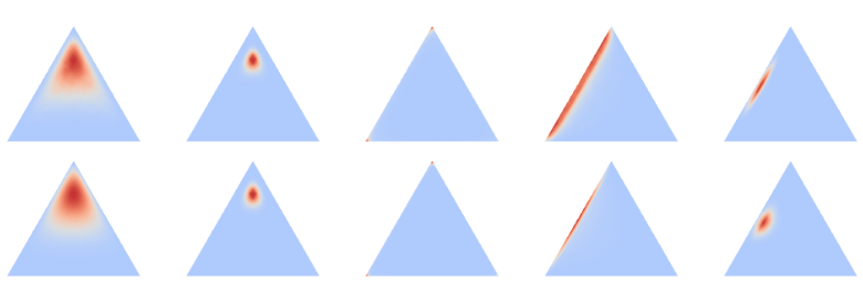
We firstly find that the LB is an imperfect but sufficiently good map, i.e. we can see small differences but the two rows look mostly similar. Secondly, the parameters of the Gaussian have been chosen to stress important ideas. Case 1 and 2 (from left to right) have the same mean but different covariance matrices. This further emphasizes the need for a Bayesian interpretation of ML as uncertainty matters here. Using the mode or mean as point estimate would treat 1 and 2 similarly even though the respective uncertainties are clearly different. Scenarios 3, 4, and 5 show similar means with increasing uncertainty. This case was chosen to show that this change of uncertainty in the original Gaussian is successfully mapped through the Laplace Bridge to further convince us that it is worth considering for practical applications.
LB applied to BNNs
In the context of Bayesian Neural Networks, one possibility to generate your distribution of the outputs is to estimate a Gaussian of the logits, then draw samples from it and apply the softmax to each sample individually. There are other possibilities to estimate an output distribution but sampling is commonly used as it’s a cheap and easy-to-use method. Applying a softmax to a Gaussian does not yield a closed-form solution and drawing samples is therefore the only possible way to estimate the true posterior. However, since we want to transform a distribution in logit-space \(\mathbb{R}^D\) to a distribution in probability space \(\mathbb{P}^{D}\) using the Laplace Bridge seems like a good option to get rid of the expensive sampling step. To get a visual intuition where exactly we apply the LB consider the following figure once more.
The important thing to keep in mind is that the Laplace Bridge works on all kinds of BNNs as long as they produce a Gaussian over the logits. That means it could be applied to Variational Inference or sampling-based schemes like ensembles as well. It is, therefore, a very light-weight addition to the network and can be easily applied in most circumstances.
Limitations and corrections
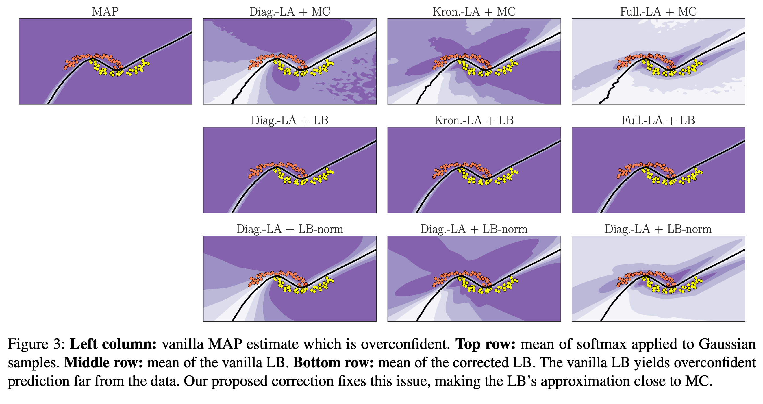
While getting deeper and deeper into the LB, I started to notice more and more failure cases. Specifically, when the variance of the Gaussian was very large, the corresponding Dirichlet got overconfident. Intuitively, this also makes sense. If you look at the definition of the Laplace Bridge from \((\mu, \Sigma)\) to \(\alpha\), you can see that the variance terms \(\Sigma_{kk}\) have a linear influence on \(\alpha_k\) while \(\mu_k\)’s influence is exponential. If you draw samples from a Gaussian and apply the softmax, this difference in influence is not given. This means the LB becomes worse for large uncertainty. We discuss this limitation and its origins in more detail in the paper.
We suggest a correction to counteract this behavior by basically rescaling every \(\mu\) and \(\Sigma\) back to a range of values where the LB works well (see paper for math). You can see an example of the vanilla LB and the corrected version in the following figure.
Experiments
From the framing of the paper so far, I think three questions arise quite naturally: a) How good is the approximation in the context of BNNs?, b) How much faster is it compared to sampling?, and c) Are there use-cases for a Dirichlet distribution that do not exist for a distribution of softmax-Gaussian samples. The experiments aim to answer these questions in chronological order.
Out-of-Distribution Experiments
Naturally, when we have a new approximation, we want to know how good its quality is. Since one of the main use-cases of output distributions is out-of-distribution (OOD) detection we tested it first. We use a Laplace approximation of the network to generate our Gaussians over the logits. This becomes computationally expensive very quickly for larger networks and we, therefore, apply a last-layer Laplace approximation for all but the (F-, K-, not-)MNIST experiments. The last-layer Laplace approximation has been shown to yield pretty good uncertainty estimates (see e.g. Brosse et al. 2020) but is also very much in the spirit of this paper as we want to get a reasonably good uncertainty estimate very quickly and therefore prioritize speed.
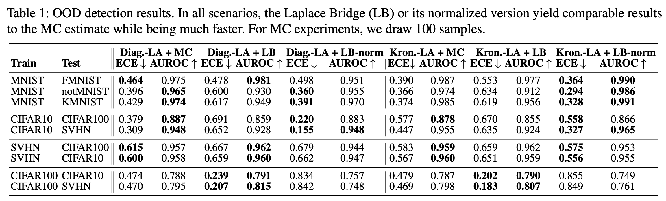
We compare the mean of the Dirichlet from the LB on a standard benchmark suite for OOD detection in multiple scenarios. Firstly, we compare a diagonal approximation of the Hessian vs. a kronecker-factorized (Kron) approximation. As expected, the Kron is better than the diagonal one. Secondly, we compare sampling (MC) vs. the vanilla LB and LB with correction (LB-norm). We find that either the LB or LB-norm can compete with sampling most of the time while being much faster.
We ran multiple other experiments to compare the LB with other methods (see paper for numbers).
Firstly, we compared it to the extended probit approximation which is another way to approximate the softmax-Gaussian integral. The LB outperforms the extended probit approximation consistently.
Secondly, we compared the LB to Prior networks (PNs) since both yield Dirichlet distributions as output. The PNs outperform the LB results very consistently. However, I don’t think this is a problem for the LB since PNs are a method to train NNs and the LB is used on top of an already trained NN. Therefore, I think this result is not that relevant for practitioners.
Thirdly, we compared a last-layer approximation of the Hessian with an all-layer approach. We find that, as expected, the all-layer approach is slightly more accurate than the last-layer one. However, given that the main goal of the LB is speed, we think the last-layer approach makes more sense for almost all realistic use-cases.
Timing Experiments
As our main priority is achieving fast predictive uncertainty in BNNs we want to find out what the trade-off between accuracy and speed of the LB is. For that, we consider the KL divergence between the Dirichlet resulting from the LB and the true distribution to the KL divergence from samples to the true distribution where the true distribution is approximated by MCMC-sampling with 100k samples. We compare the KL divergences for three different samples of Gaussian distributions depending on the number of samples (left) and the actual wall-clock time needed for the computations (right)
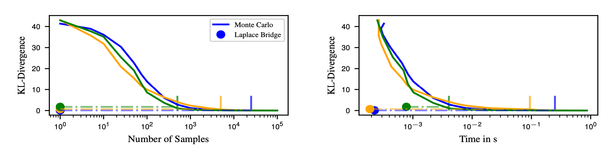
We find that it takes between 750 and 10k samples to achieve the same KL divergence to the true distribution as the LB and around 100 times much longer to get the same accuracy. This further indicates that we should use the LB if our goal is to maximize speed while accepting a small but fixed drop in quality.
Another question is how much this speed-up does in the grand scheme of things. After all, if the last step would only make up one percent of the entire costs there would be no large benefit in improving it. To test these timings we measure the time it takes to do one forward pass and compare it with the time for the final prediction for sampling and the LB, respectively. We use a ResNet-18 with last-layer Laplace approximation for the CIFAR10 dataset. We compare the times it takes to draw 10, 100, or 1000 samples from the Gaussian.
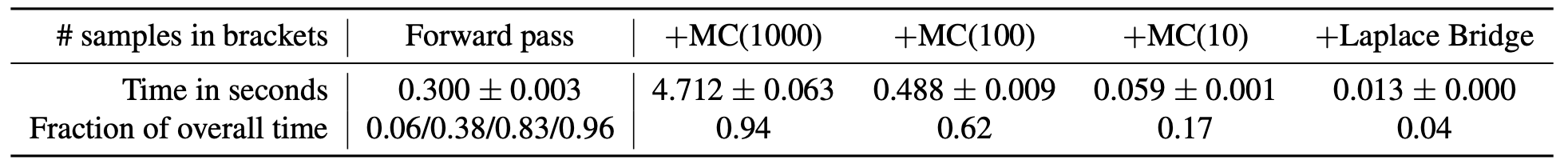
We can already see that the sampling process is not negligible for the timing of the entire prediction. Taking 1000 samples makes up 94 percent of the entire time and taking 10 samples still takes 17 percent. The Laplace Bridge, in comparison, only takes up 4 percent. Even though we are only talking about seconds or even just milliseconds, there is a range of applications that operate on small time scales. In self-driving cars, for example, this could be the difference between a close call and an accident.
Lastly, one could assume that computing the mean and covariance matrix for the Laplace approximation is too costly and this approach is therefore overall not applicable. However, with fast computational tools such as BACKpack or Laplace Torch, which are fast automatic differentiation tools on top of PyTorch, we can compute the uncertainties at the cost of one backward pass. In our setup, we train a ResNet-18 on CIFAR10 in 130 epochs, which takes 71 minutes and 30 seconds. Computing the uncertainties is done in 29 seconds and therefore a very small price to pay for the benefit of having full distributions over the outputs.
Uncertainty-aware top-k
The performance of image classification networks in the context of ImageNet which is a large dataset with 1000 classes is often measured along a top-1 and a top-5 metric. While it seems plausible to not only look at the highest-rated estimate but also the following ones the specific number of five seems both arbitrary and pretty inflexible. We can, for example, easily think of situations where this is either too large or too small of a number. Imagine a scenario in which your network receives the image of a fish and decides it is one of the ten possible fish species available in the training data but can’t decide between them. Then it is a coin flip if the correct class is in your top-5. If, on the other hand, the network is pretty sure that the image either belongs to the class “eagle” or “hawk” then the three remaining classes within the top-5 don’t add any value to the classification. What we would want is a more flexible solution that includes the network’s own uncertainty estimates to create a border between possible candidates and unlikely estimates. We use the Dirichlet resulting from the LB to construct an uncertainty-aware top-\(k\) metric. Marginal distributions of the Dirichlet are Dirichlets again and can be computed in closed-form by \(\mathrm{Beta}(\alpha_i, \sum_{j\neq i} \alpha_j)\). Importantly, this means we can estimate a marginal Beta distribution (the 1D special case of the Dirichlet) for every single class in a given prediction. We can use the overlap between sorted estimates to decide whether they are inside or outside of the top-k estimate similar to T-tests or their Bayesian equivalents. For example, we could say that all classes that have a five percent overlap with the top class are inside the estimate. This concept is illustrated with the following figure.
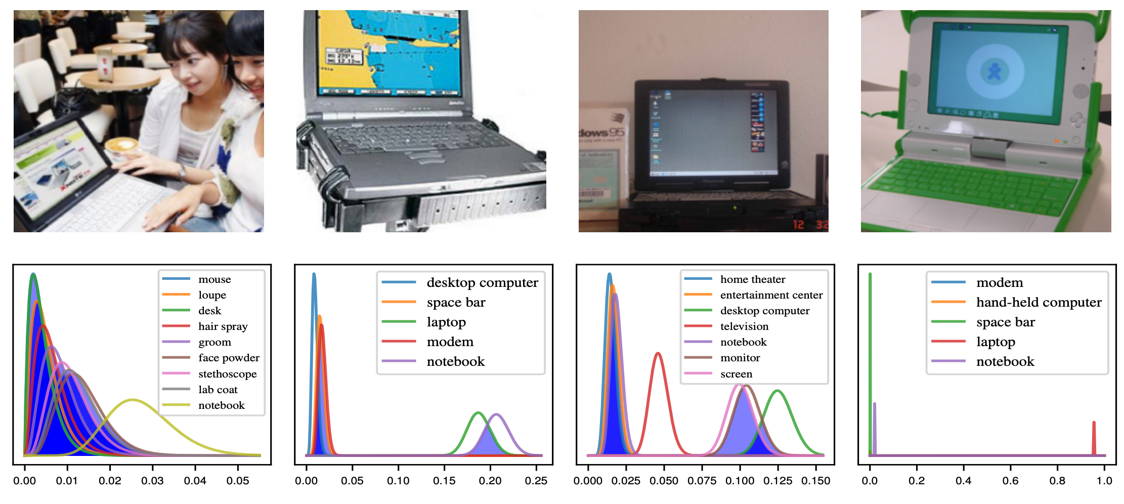
As you can see these four images yield vastly different top-\(k\) estimates. From left to right we have a top-\(1000\) estimate where all classes overlap sufficiently to say we don’t really have a confident prediction, a top-\(2\) estimate, a top-\(3\) estimate, and a top-\(1\) estimate. In all cases using a top-\(5\) estimate as the default would be either insufficient or wasteful. As the above examples have been cherry-picked to illustrate the point we should also look at the distribution of \(k\) for the top-\(k\) estimates.
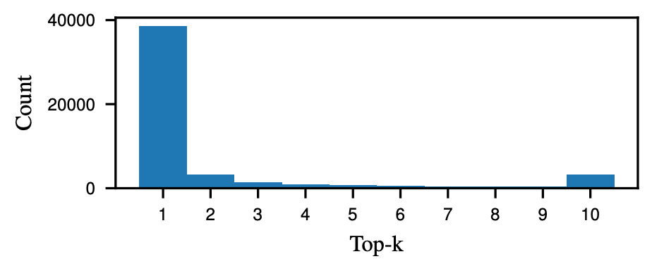
About 40k of the 50k images fall into the top-\(1\) bin as the network is pretty confident in its prediction for the vast majority of cases. There are some top-\(2\) and even less top-\(3\) estimates whenever there is ambiguity and the last bin with top-\(10\) estimates that represent the ``I don’t know’’ class of predictions. I think this shows that using a static value of \(k\) for predictions does not accurately reflect the uncertainty of the underlying network. In some sense it already knows that the top-1 estimate might be wrong but we keep asking the wrong question.
Conclusions
The Laplace Bridge for BNNs is not going to revolutionize Bayesian inference in Neural Networks but it might be useful in some cases. Replacing an expensive part of the prediction pipeline with something much faster at some cost in approximation quality and getting a full distribution could be helpful in some practical applications. Additionally, it is really simple to apply to any network that has a Gaussian distribution over its logits and you can check out the GitHub repo if you want to try it out yourself.
One last note
If you want to get informed about new posts follow me on Twitter.
If you have any feedback regarding anything (i.e. layout, code, or opinions) please tell me in a constructive manner via your preferred means of communication.